| Contents |
|---|
| The Haar Prediction Function |
| A Linear Approximation Prediction Function |
| A Polynomial Approximation Prediction Function |
| Quality of the Approximation |
| Predict Wavelet Software in Java |
The wavelet Lifting Scheme is a method for decomposing wavelet transforms into a set of stages. Lifing scheme algorithms have the advantage that they do not require temporary arrays in the calculation steps, as is necessary for some versions of the Daubechies D4 wavelet algorithm.
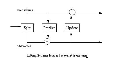
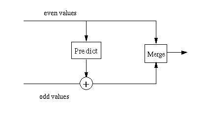
The simplest version of a forward wavelet transform expressed in the Lifting Scheme is shown below in Figure 1. The predict step is the subject of this web page, which will considered in isolation. The predict step calculates the wavelet function in the wavelet transform. This is a high pass filter. The update step calculates the scaling function, which results in a smoother version of the data. The complete lifting scheme is discussed on the Basic Lifting Scheme web page. This web page is intended to provide background for this discussion.
Figure 1
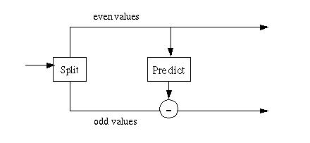
Figure 2 shows the ur-Lifting Scheme transform, consisting of two steps:
Split step: divide the input data into odd and even elements. In a finite data set the odd elements are moved to the second half of the array, leaving the even elements in the first half.
Predict step: predict the odd elements from the even elements.
Figure 2
One way to view the predict step is through the lens of data compression. If our objective is to compress a set of data and the odd elements can be absolutely predicted from the even elements using the equation
odd = even * 2;
the odd elements can be replaced by zero. If we apply a compression algorithm like run length encoding the odd elements will be reduced to a count and zero, compressing the original data set by almost 50%. If the data set consists of points on a line, then it can be reduced to something close to a single element and the length of the data set. In most cases the data set is more complex and it cannot be entirely represented by a starting condition, a length and an equation. However, a more compact representation might be arrived at by approximating the data in a local region using a function. The predict stage replaces an odd element with the difference between the odd element a function calculated from the even elements. The simplest example of such a predict stage takes a single even element as its argument to calculate the predicted value of the odd element:
oddj+1,i = oddj,i - P(evenj,k)
Here the function P() is the predict function. Wavelet algorithms are recursive, so the recursive step j generates data for the next recursive step j+1. The subscript i indexes the odd part of the array. The subscript k indexes the even part of the array.
One of the simplest predict functions is simply
oddj+1,i = evenj,k
If the split step had not divided the odd and even elements, the predict step predicts that the odd value is equal to its even predecessor.
ai+1 = ai;
The predict step replaces the odd elements with the difference between the actual odd value and the predicted value:
oddj+1,i = oddj,i - evenj,k
If the data shows a trend (in the language of statistics the data shows autocorrelation), then the odd element can be predicted from the even element, to some degree. As a result, the difference between the odd element and its predictor (the even element) will be smaller than the odd element itself. Smaller values can be represented in fewer bits, so some level of compression can be achieved.
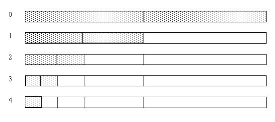
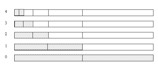
The process of "predicting" the odd elements from the even elements is recursive, as long as the number of data elements is a power of two. After the first pass, the odd (upper) half of the array will contain the differences between the prediction and the original odd element values. The next recursive pass divides the lower half of the array into odd and even halves. The difference between the prediction and the odd element value is stored in the new odd half. The recursive passes continue until the last step where a single odd element is predicted from a single even element. This is shown in Figure 3 below.
Figure 3
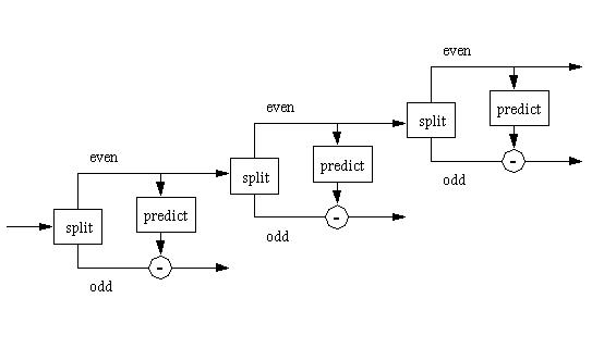
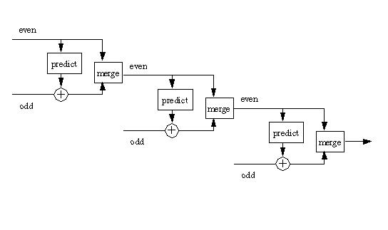
Another way to view this is as a chain of split/predict steps, where the even elements from one step become the input for the next step.
Figure 4
The closer the predict function fits the data the smaller the differences will be. A prediction function that closely fits the data will allow the result of the predict wavelet to be represented in fewer bits, so there will be a higher level of compression.
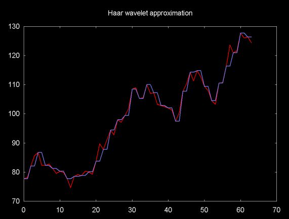
The prediction function
oddi = evenk
results in a function with a series of flat steps formed by lines
between the even and odd elements. This function is known as the Haar
wavelet function. Figure 5 is a plot of a financial time series
(e.g., set of stock close prices), shown in red, graphed with the Haar
function, shown in blue. The differences which will be stored in the
odd elements when the predict wavelet is calculated are the
differences between the time series and the Haar function.
Figure 5
The inverse predict wavelet transform is the mirror of the forward transform. However, rather than subtracting the prediction from the odd element, the prediction is added. This is shown in Figure 6. The merge step merges the odd an even elements back together (e.g., the merge step is the inverse of the split step).
Figure 6
The forward transform works on data sizes that are decreasing powers of two. The inverse transform works on increasing powers of two (i.e., 2, 4, 8, 16...). This is shown in Figure 7, below.
Figure 7
The inverse transform can be viewed as a chain of predict/merge steps, where the merged data becomes the input for the even elements in the next step. This is shown in Figure 8 below.
Figure 8
There are an infinite number of predict functions which can be used. Ideally the predict function used should closely fit the input data within a defined region. In the case of a jagged time series, like a financial time series (or a set of weather temperature changes, sampled over different days), it might be better to predict that the odd element lies on a line between two even elements:
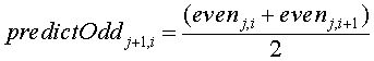
The graph in Figure 9 shows a financial time series (in red) and a line where the odd elements are at the mid-point between the even elements. Note that the predict line more closely fits the data than does the Haar wavelet predict function. The closer the function fits a local part of the data the smaller the differences stored in the odd elements will be. Small values can be represented in fewer bits, so a higher degree of compression will result.
Figure 9

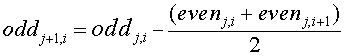
If the predict function is that the odd element is at the mid-point between the even elements, the difference stored for each odd element will be
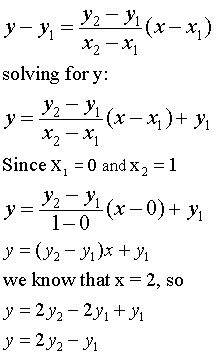
There is a minor edge issue with the line wavelet. Wavelets operate on data with a power of two elements. So the last element in the data set will be an odd element. There is no evenj,i+1 element that brackets this element. For this last element the predict step "predicts" that the odd element lines on a line defined by its two even predecessors.
The calculation of this extra value "pretends" that the last two even values in the data series are at the x-axis coordinates 0 and 1, respectively. The extra value will be at located at the x-axis coordinate 2. The calculation of the y-axis coordinate uses the "two-point" equation.
The "two-point equation" for a line given x1, y1 and x2, y2 is
If the data set that we are trying to fit is smooth, it might be better fit with a polynomial than with the flat Haar lines or the sloped lines of the mid-point predictor described above. For example, given the four even points
evenj,k-1, evenj,k, evenj,k+1, evenj,k+2
we can use polynomial interpolation to predict the the odd point between evenj,k, evenj,k+1, using the four even points between k-1 and k+2.
Polynomial interpolation is implemented via 4-point Lagrange polynomial interpolation. Given four even points, even0, even1, even2, even3 (which we pretend are located a x-coordinates 0, 1, 2, 3, regardless of the actual x-coordinates), an odd point is interpolated (predicted) between even1 and even2. The interpolated point will be located at 1.5 (for the moment I'll pretend that I'm a mathematician and I'm dealing with an infinite series of data, so there are no special cases at the edges).
To calculate the interpolated point at even0, even1, even2, even3 the equation below is used.
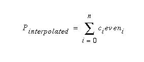
For 4-point Lagrange interpolation this is
Pinterpolated = c0even0 + c1even1 + c2even2 + c3even3
For a given n-point polynomial interpolation of a point at x, the coefficients are constant and can be calculated once. For an interpolated point at x (in this case, x = 1.5), a set of coefficients c0, c1, c2, c3 are calculated using the Lagrange equation shown below
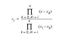
This equation is implemented by the lagrange function shown below. This function is passed x, the point to be interpolated and N, the number of points. The function assumes that the points d0 ... dn are located at the x-coordinates 0 ... N-1.
void lagrange( const double x, const int N, double c[] )
{
  double num, denom;

  for (int i = 0; i < N; i++) {
    num = 1;
    denom = 1;
    for (int k = 0; k < N; k++) {
      if (i != k) {
        num = num * (x - k);
        denom = denom * (i - k);
      }
    } // for k
    c[i] = num / denom;
  } // for i
}
So far the point that is being interpolated is in the middle of the four even points (at the x-coordinate 1.5). This will not interpolate the odd points at the start and end of the data set. At the start of the data set the first odd point is interpolated between the first and second even points. This odd point is located at 0.5 (relative to the even points). At the end of the data set (the right side), the last two odd points will be located 2.5 and 3.5.
Figure 10 shows how even points from the data series are logically viewed as points located at x-coordinates 0, 1, 2, 3. The circles represent the odd points which are located between the even points.
Figure 10
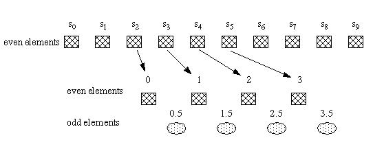
At the end of the recursive wavelet calculation for polynomial interpolation, there will be only two even points. The last two odd points are "predicted" using 2-point polynomial interpolation (e.g., linear interpolation).
As shown above, the coefficients can be calculated in advance. This is shown in the table below:
4-point interpolation
| interpolation @ x-coordinate |
c0 | c1 | c2 | c3 |
|---|---|---|---|---|
| 0.5 | 0.3125 | 0.9375 | -0.3125 | 0.0625 |
| 1.5 | -0.0625 | 0.5625 | 0.5625 | -0.0625 |
| 2.5 | 0.0625 | -0.3125 | 0.9375 | 0.3125 |
| 3.5 | -0.3125 | 1.3125 | -2.1875 | 2.1875 |
2-point interpolation
| interpolation @ x-coordinate |
c0 | c1 |
|---|---|---|
| 0.5 | 0.5000 | 0.5000 |
| 1.5 | -0.5000 | 1.5000 |
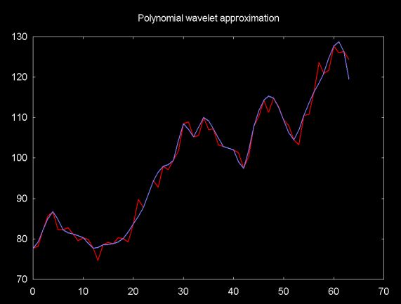
Figure 11 shows a 4-point polynomial fit for the financial time series. The red line plots the time series, the blue line the polynomial fit. The even points correspond to the time series. The odd points are the polynomial interpolation values.
Figure 11
The difference between the predicted value and the actual odd value is stored in the odd element. The better the predictor, the smaller the difference. So one way to look at the quality of the prediction function is to look at the distribution of differences. This is shown in Figures 12, 13 and 14, below. These plots show the histogram of the absolute value of the difference between the predicted value and the actual odd element value.
Figure 12, Distribution of Haar wavelet function differences
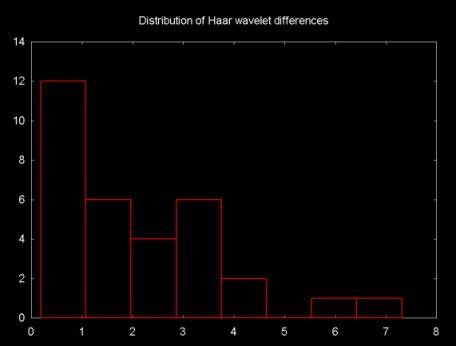
Figure 13
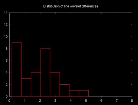
Figure 14
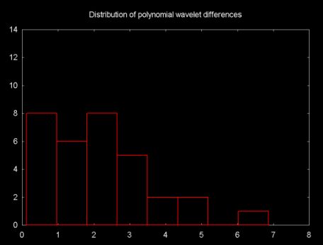
The differences between the distributions is relatively small. The "line wavelet" shows the best fit for the financial time series. There is very little difference between the Haar and the polynomial interpolation wavelet.
Java source code implementing the Haar, line and polynomial interpolation algorithms described above can be downloaded from the web page linked to above.
Basic Lifting Scheme Wavelets (this web page is the successor to this web page).
Wavelet Lifting Scheme main page (the parent of this web page)
Ian Kaplan
November 2001
Revised:
