
The Daubechies wavelet transform is named after its inventor (or would it be discoverer?), the mathematician Ingrid Daubechies. The Daubechies D4 transform has four wavelet and scaling function coefficients. The scaling function coefficients are
Each step of the wavelet transform applies the scaling function to the the data input. If the original data set has N values, the scaling function will be applied in the wavelet transform step to calculate N/2 smoothed values. In the ordered wavelet transform the smoothed values are stored in the lower half of the N element input vector.
The wavelet function coefficient values are:
g0 = h3
g1 = -h2
g2 = h1
g3 = -h0
Each step of the wavelet transform applies the wavelet function to the input data. If the original data set has N values, the wavelet function will be applied to calculate N/2 differences (reflecting change in the data). In the ordered wavelet transform the wavelet values are stored in the upper half of teh N element input vector.
The scaling and wavelet functions are calculated by taking the inner product of the coefficients and four data values. The equations are shown below:
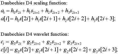
Each iteration in the wavelet transform step calculates a scaling function value and a wavelet function value. The index i is incremented by two with each iteration, and new scaling and wavelet function values are calculated. This pattern is discussed on the web page A Linear Algebra View of the Wavelet Transform.
In the case of the forward transform, with a finite data set (as opposed to the mathematician's imaginary infinite data set), i will be incremented until it is equal to N-2. In the last iteration the inner product will be calculated from calculated from s[N-2], s[N-1], s[N] and s[N+1]. Since s[N] and s[N+1] don't exist (they are byond the end of the array), this presents a problem. This is shown in the transform matrix below.
Daubechies D4 forward transform matrix for an 8 element signal
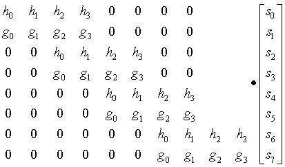
Note that this problem does not exist for the Haar wavelet, since it is calculated on only two elements, s[i] and s[i+1].
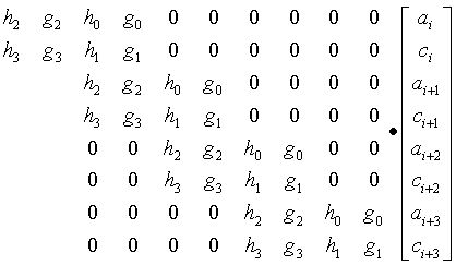
A similar problem exists in the case of the inverse transform. Here the inverse transform coefficients extend beyond the beginning of the data, where the first two inverse values are calculated from s[-2], s[-1], s[0] and s[1]. This is shown in the inverse transform matrix below.
Daubechies D4 inverse transform matrix for an 8 element transform result
Three methods for handling the edge problem:
Treat the data set as if it is periodic. The beginning of the data sequence repeats folling the end of the sequence (in the case of the forward transform) and the end of the data wraps around to the beginning (in the case of the inverse transform).
Treat the data set as if it is mirrored at the ends. This means that the data is reflected from each end, as if a mirror were held up to each end of the data sequence.
Gram-Schmidt orthogonalization. Gram-Schmidt orthoganalization calculates special scaling and wavelet functions that are applied at the start and end of the data set.
Zeros can also be used to fill in for the missing elements, but this can introduce significant error.
The Daubechies D4 algorithm published here treats the data as if it were periodic. The code for one step of the forward transform is shown below. Note that in the calculation of the last two values, the start of the data wraps around to the end and elements a[0] and a[1] are used in the inner product.
   protected void transform( double a[], int n )
   {
      if (n >= 4) {
         int i, j;
         int half = n >> 1;

         double tmp[] = new double[n];

         i = 0;
         for (j = 0; j < n-3; j = j + 2) {
            tmp[i]      = a[j]*h0 + a[j+1]*h1 + a[j+2]*h2 + a[j+3]*h3;
            tmp[i+half] = a[j]*g0 + a[j+1]*g1 + a[j+2]*g2 + a[j+3]*g3;
            i++;
         }

         tmp[i]      = a[n-2]*h0 + a[n-1]*h1 + a[0]*h2 + a[1]*h3;
         tmp[i+half] = a[n-2]*g0 + a[n-1]*g1 + a[0]*g2 + a[1]*g3;

         for (i = 0; i < n; i++) {
            a[i] = tmp[i];
         }
      }
   } // transform
The inverse transform works on N data elements, where the first N/2 elements are smoothed values and the second N/2 elements are wavelet function values. The inner product that is calculated to reconstruct a signal value is calculated from two smoothed values and two wavelet values. Logically, the data from the end is wrapped around from the end to the start. In the comments the "coef. val" refers to a wavelet function value and a smooth value refers to a scaling function value.
   protected void invTransform( double a[], int n )
   {
      if (n >= 4) {
        int i, j;
        int half = n >> 1;
        int halfPls1 = half + 1;

        double tmp[] = new double[n];

        //      last smooth val  last coef.  first smooth  first coef
        tmp[0] = a[half-1]*Ih0 + a[n-1]*Ih1 + a[0]*Ih2 + a[half]*Ih3;
        tmp[1] = a[half-1]*Ig0 + a[n-1]*Ig1 + a[0]*Ig2 + a[half]*Ig3;
        j = 2;
        for (i = 0; i < half-1; i++) {
          //     smooth val     coef. val       smooth val     coef. val
          tmp[j++] = a[i]*Ih0 + a[i+half]*Ih1 + a[i+1]*Ih2 + a[i+halfPls1]*Ih3;
          tmp[j++] = a[i]*Ig0 + a[i+half]*Ig1 + a[i+1]*Ig2 + a[i+halfPls1]*Ig3;
        }
        for (i = 0; i < n; i++) {
          a[i] = tmp[i];
        }
      }
   }
I do not agree with the policy of the authors of Numerical Recipes prohibiting redistribution of the source code for the Numerical Recipes algorithms. With most numerical algorithm code, including wavelet algorithms, the hard part is understanding the mathematics behind the algorithm. There is not that much "intellectual property" in the source code. In contrast to the Numerical Recipes code, you may use the wavelet code published here for what ever purpose you desire, including redistribution in source form. All I ask is that you credit me with authorship.
I recommend using the "save as" feature of your browser to save the C++ and Java source files (I'm not sure how to reliably suppress viewing and force download with all browsers).
The Daubechies D4 algorithm as a C++ class
Doxygen generated documentation for the C++ version of the Daubechies D4 algorithm. This documentation was generated with this Doxygen configuration file.
The Daubechies D4 algorithm as a Java class
The wavelet Lifting Scheme was developed by Wim Sweldens and others. Wavelet Lifting Scheme algorithms have several advantages. They are memory efficients and do not require a temporary array as the version of the Daubechies D4 transform above does. As the diagrams below show, the inverse transform is the mirror of the forward transform, when additions exchanged for subtractions. The Lifting Scheme is discussed at some length here
Ripples in Mathematics describes a lifting scheme version of the Daubechies D4 transform. Lifting Scheme wavelet transforms are composed of Update and Predict steps. In this case a normalization step has been added as well. One forward transform step is shown in the diagram below.
Forward transform step of the lifting scheme version of the Daubechies D4
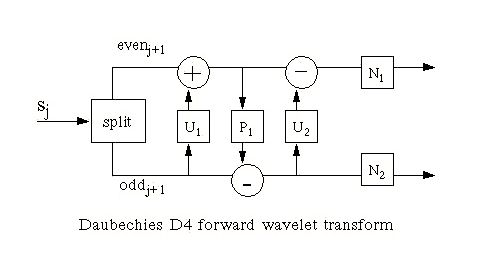
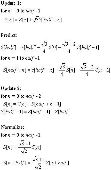
The split step divides the input data into even elements which are stored in the first half of an N element array section ( S0 to Shalf-1) and odd elements which are stored in the second half of an N element array section (Shalf to SN-1). In the forward transform equations below the expression S[half+n] references an odd element and S[n] references an even element. Although the diagram above shows two normalization steps, in practice they are folded into a single function.
Forward transform step equations
One of the elegant features of Lifting Scheme versions of the wavelet transform is the fact that the inverse transform is a mirror of the forward transform, which addition and subtraction operations interchanged.
Inverse transform step of the lifting scheme version of the Daubechies D4
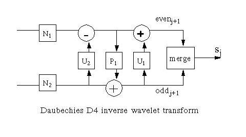
The merge step interleaves elements from the even and odd halves of the vector (e.g., even0, odd0, even1, odd1, ...).
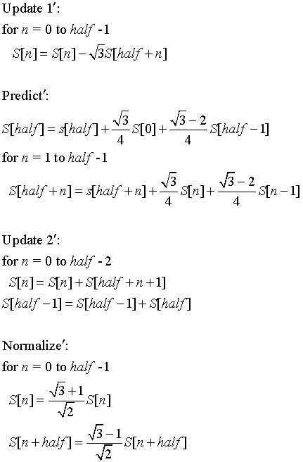
As the diagram above shows, the inverse transform equations have addition and subtraction operations interchanged. The inverse normalization step works because, as noted in Ripples
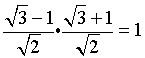
Inverse transform step equations
The scaling function (which uses the hn coefficients) produces N/2 elements that are a smoother version of the original data set. In the case of the Haar transform, these elements are a pairwise average. Each stage of the Haar transform preserves the following equation.
http://www.bearcave.com/misl/misl_tech/wavelets/lifting/average.jpg
This is sometimes referred to as the zeroth moment. The last step of the Haar transform calculates one scaling value and one wavelet value. In the case of the Haar transform, the scaling value will be the average of the input data.
The equation above is not "honored" by the versions of the Daubechies transform described here. If we apply the Lifting Scheme version of the Daubechies forward transform to the data set
  S = {32.0, 10.0, 20.0, 38.0, 37.0, 28.0, 38.0, 34.0,
       18.0, 24.0, 18.0, 9.0, 23.0, 24.0, 28.0, 34.0}
we get the following ordered wavelet transform result (printed to show the scaling value, followed by the bands of wavelet coefficients)
103.75  <=== scaling value
-11.7726
3.5887 21.9969
17.7126 -1.5744 -1.0694 3.6405
-10.6945 8.0048 -6.3225 -4.3027 9.0723 -3.0018 -3.3021 1.3542
The final scaling value in the Daubechies D4 transform is not the average of the data set (the average of the data set is 25.9375), as it is in the case of the Haar transform. This suggests to me that the low pass filter part of the Daubechies transform (i.e., the scaling function) does not produce as smooth a result as the Haar transform.
The tar file daubechies.tar below contains three files:
daubbook.java
This version of the Lifting Scheme Daubechies D4 transform is modeled on the C code in Ripples in Mathematics, but without the temporaries. All lifting steps are included in a single transform step.
lift/liftbase.java
The Java lift package contains a number of Lifting Scheme algorithms, including the Daubechies D4 transform. The liftbase class is an abstract class that defines the basic structure of the lifting scheme algorithm. This class provides the split and merge functions, which all lifting scheme wavelets use.
lift/daubechies.java
The Lifting Scheme version of the Daubechies D4 transform described in Ripples in Mathematics. This class is derived from the liftbase abstract class.
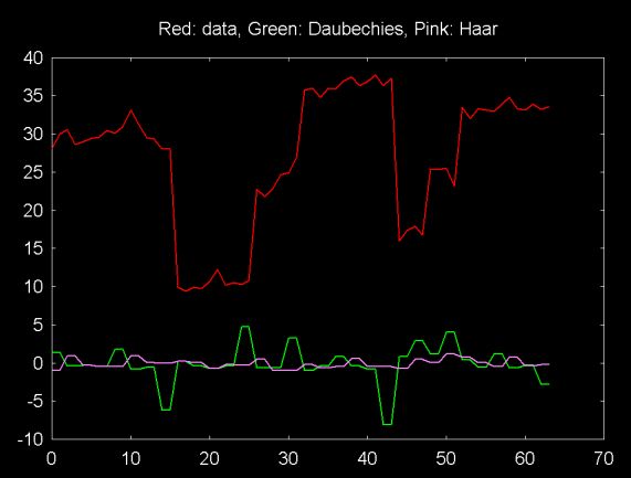
When I first started studying wavelets, one of the many questions I had was "How does one decide which wavelet algorithm to use?" There is no absolute answer to this question. The choice of the wavelet algorithm depends on the application. The Haar wavelet algorithm has the advantage of being simple to compute and easier to understand. The Daubechies D4 algorithm has a slightly higher computational overhead and is conceptually more complex. As the matrix forms of the Daubechies D4 algorithm above show, there is overlap between iterations in the Daubechies D4 transform step. This overlap allows the Daubechies D4 algorithm to pick up detail that is missed by the Haar wavelet algorithm.
The red line in the plot below shows a signal with large changes between even and odd elements. The pink line plots the largest band of Haar wavelet coefficients (e.g., the result of the Haar wavelet function). The green line plots the largest band of Daubechies wavelet coefficients. The coefficient bands contain information on the change in the signal at a particular resolution.
In this version of the Haar transform, the coefficients show the average change between odd and even elements of the signal. Since the large changes fall between even and odd elements in this sample, these changes are missed in this wavelet coefficient spectrum. These changes would be picked up by lower frequency (smaller) Haar wavelet coeffient bands.
The overlapped coefficients of the Daubechies D4 transform accurately pick up changes in all coefficient bands, including the band plotted here.
Ripples in Mathematics: the Discrete Wavelet Transform by Arne Jense and Anders la Cour-Harbo, Springer, 2001
The material on this web page relies heavily on Ripples in Mathematics (although all errors are mine). The Lifting Scheme version of the Daubechies D4 transform is lifted from this book. Ripples is the best book I've been able to find on wavelets, from an implementation point of view.
The equations on this Web pages (and other web pages) where set using MathType.
Ian Kaplan, July 2001
This web pages was completely rewritten in January 2002
Revised:
