Wavelet algorithms are recursive. The output of one step of the algorithm becomes the input for the next step. The initial input data set consists of 2n elements. Each successive step operates on 2n-i elements, were i = 1 ... n-1. For example, if the initial data set contains 128 elements, the wavelet tranform will consist of seven steps on 128, 64, 32, 16, 8, 4, and 2 elements.
On this web page stepj+1 follows stepj. If element i in step j is being updated, the notation is stepj,i. The forward lifting scheme wavelet transform divides the data set being processed into an even half and an odd half. In the notation below eveni is the index of the ith element in the even half and oddi is the ith element in the odd half (I'm pretending that the even and odd halves are both indexed from 0). Viewed as a continuous array (which is what is done in the software) the even element would be a[i] and the odd element would be a[i+(n/2)].
Another way to refer to the recursive steps is by their power of two. This notation is used in Ripples in Mathematics. Here stepj-1 follows stepj, since each wavelet step operates on a decreasing power of two. This is a nice notation, since the references to the recursive step in a summation also correspond to the power of two being calculated.
The previous section, Predict Wavelets, discusses a Lifting Scheme proto-wavelet that I call the predict wavelet. Like all lifting scheme wavelets the predict wavelet transform starts with a split step, which divides the data set into odd and even elements. The predict step uses a function that approximates the data set. The difference between the approximation and the actual data replaces the odd elements of the data set. The even elements are left unchanged and become the input for the next step in the transform. The predict step, where the odd value is "predicted" from the even value is described by the equation
oddj+1,i = oddj,i - P( evenj,i )
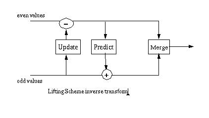
The inverse predict transform adds the prediction value to the odd element (reversing the prediction step of the forward transform). In the inverse transform the predict step is followed by a merge step which interleaves the odd and even elements back into a single data stream.
The simple predict wavelets are not useful for most wavelet applications. The even elements that are used to "predict" the odd elements result from sampling the original data set by powers of two (e.g., 2, 4, 8...). Viewed from a compression point of view this can result in large changes in the differences stored in the odd elements (and less compression). One of the most powerful applications for wavelets is in the construction of filters. The "down sampling" in the predict wavelets does not provide an approximation of the data at each step, which is one of the requirements for filter design.
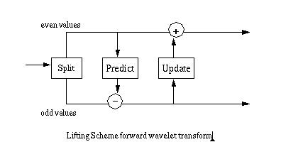
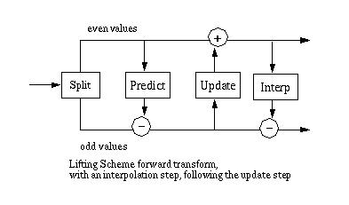
The update step replaces the even elements with an average. This results in a smoother input for the next step of the next step of the wavelet transform. The odd elements also represent an approximation of the original data set, which allows filters to be constructed. A simple lifting scheme forward transform is diagrammed in Figure 1.
Figure 1
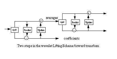
The update phase follows the predict phase. The original value of the odd elements has been overwritten by the difference between the odd element and its even "predictor". So in calculating an average the update phase must operate on the differences that are stored in the odd elements:
evenj+1,i = evenj,i + U( oddj+1,i )
In the lifting scheme version of the Haar transform, the prediction step predicts that the odd element will be equal to the even element. The difference between the predicted value (the even element) and the actual value of the odd element replaces the odd element. For the forward transform iteration j and element i, the new odd element, j+1,i would be
oddj+1,i = oddj,i - evenj,i
In the lifting scheme version of the Haar transform the update step replaces an even element with the average of the even/odd pair (e.g., the even element si and its odd successor, si+1):
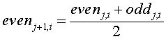
The original value of the oddj,i element has been replaced by the difference between this element and its even predecessor. Simple algebra lets us recover the original value:
oddj,i = evenj,i + oddj+1,i
Substituting this into the average, we get
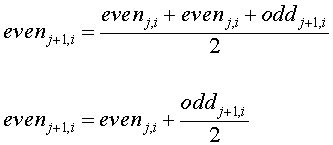
The averages (even elements) become the input for the next recursive step of the forward transform. This is shown in Figure 2, below.
Figure 2
The number of data elements processed by the wavelet transform must be a power of two. If there are 2n data elements, the first step of the forward transform will produce 2n-1 averages and 2n-1 differences (between the prediction and the actual odd element value). These differences are sometimes referred to as wavelet coefficients. Figure 3 shows a 4-steps forward wavelet transform on a 16-element data set.
Figure 3
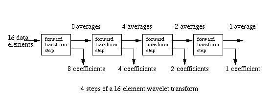
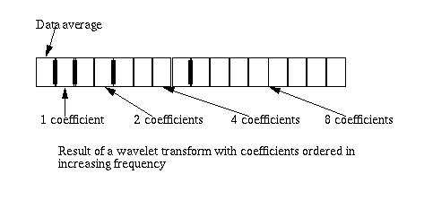
The split phase that starts each forward transform step moves the odd elements to the second half of the array, leaving the even elements in the lower half. At the end of the transform step the odd elements are replaced by the differences and the even elements are replaced by the averages. The even elements become the input for the next step, which again starts with the split phase. The result of the forward transform is shown in Figure 4. The first element in the array contains the data average. The differences (coefficients) are ordered by increasing frequency.
Figure 4
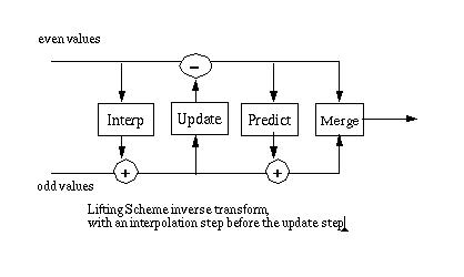
One of the elegent features of the lifting scheme is that the inverse transform is a mirror of the forward transform. In the case of the Haar transform, additions are substituted for subtractions and subtractions for additions. The merge step replaces the split step.
Figure 5
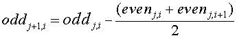
The linear interpolation function "predicts" that an odd element will be located at the mid-point of a line between its two even neighbors. The difference between the predicted value and the actual value of the odd element replaces the odd element.
For a description of the linear interpolation predict step see A Linear Approximation Prediction Function.
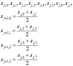
The update step replaces the even elements with an average of the data being processed (an avarage formed from even and odd elements). If here are 2n elements, there will be 2n-1 even elements, or averages. An example is shown below, where 2n = 8.
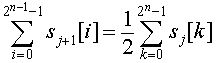
This means that the sum of the sj+1 elements is equal to the sum of the sj elements, divided by two:
There are two important features to note about the update step. The update step, like the predict step, must be invertable. In the forward transform the update value is added to the evenj,i value:
evenj+1,i = evenj,i + U( oddj+1,i )
In the inverse transform the update value is subtracted from the eveni,j value.
evenj+1,i = evenj,i - U( oddj+1,i )
The update value is calculated before the inverse predict step, so the update value must be calculated from the wavelet difference coefficients (e.g., the odd values that resulted for the forward transform predict step).
In the case of the Haar wavelet the odd values can be recovered using an equation derived from simple algebraic substitution. In the case of linear interpolation wavelets, the situation is more complex. Some journal articles and PhD theses give the equation for the update step for linear interpolation wavelets equation, without derivation. For the forwared transform this is
A rather weak derivation of the update step is included here in part to demonstrate how complex such a derivation can become for even a relatively simple predict step.
In Ripples in Mathematics the authors write
We decide to base the procedure [the calculation of the update step] on the two most recently computed differences.
In the notation I've been using on this web page the equation would be
evenj+1,i = evenj,i + A(oddj+1,i-1 + oddj+1,i)
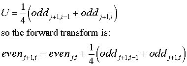
Where A is a constant. The result of the update step preserves the average, as noted above. Using something like the horrible derivation below, we can derive the value of A.
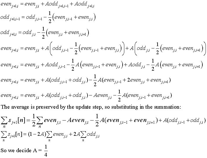
So, in summary, the forward lifting step equation is
The inverse lifting step subtracts the result of the update function from the even value.
I have included my attempt at a derivation (and there are a few leaps and, perhaps, errors in my version) to show how unwieldy it can be to arrive at an update function via derivations of this kind. If the calculation of the update step requires such difficult derivations, the generality of the wavelet lifting scheme would be severely limited.
If there is a predict function
oddj+1,i = oddj,i - P( evenj,i )
we would like to calculate the update function U( oddj+1,i ) that produces a result that, when added to eveni,j will preserve something like the average. Ideally the update function should be calculated algorithmically from the predict function. This would allow us to choose an arbitrarily complex predict function and still have a correct update step. Sadly the calculation of the update function is one of the areas that is most poorly covered in the wavelet literature.
Digital signal processing deals with filters that can remove selected parts of the signal. A high pass filter allows high frequency components to pass through, suppressing low frequency components. A low pass filter does this opposit: it allows the low frequency parts of the signal to pass through while removing the high frequency components.
The predict step replaces the odd elements with the difference between the odd elements and the predict function. The differences that replace the odd elements will reflect high frequency components of the signal. This can be viewed as a high pass filter.
The update step replaces the even elements with a local average. The result will be an approximation of the signal that is smoother than the signal at the previous level. This can be viewed as a low pass filter, since the smoother signals contains fewer high frequency components.
Any area of specialty develops its own language. This is certainly true of mathematics in general and wavelets in particular. The Lifting Scheme was developed fifteen years or so after wavelet mathematics started to be developed as a recognized area of applied mathematics. So there is small body of wavelet terminology that predates the Lifting Scheme.
The wavelet literature refers to a wavelet function. Mapped into the lifting scheme, this is the function used in the predict phase. The wavelet function is used to calculate the differences, or wavelet coefficients, and acts as the high pass filter for the odd half of the data set.
In the wavelet literature the partner to the wavelet function is the scaling function. The scaling function results in a smoother representation of the even half of the input data set. The scaling function acts as a low pass filter.
One way to side step the problem of calculating a scaling function, given a particular wavelet function, is to extend the Haar wavelet algorithm. This allows a polynomial interpolation wavelet function to be used with the Haar scaling function. This is shown in Figure 6, below. The predict and update stages are those from the Haar transform. A third polynomial interpolation stage follows these.
Figure 6
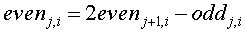
The polynomial interpolation stage calculates a "predicted" odd value from four even values (this is described at length on the related predict wavelet web page). In this case the even values are the result of the Haar scaling function (e.g., the smoothed values). The value "predicted" by polynomial interpolation is subtracted from the corresponding odd value. The odd value at this point is the difference between the original odd value and its even predecessor.
The inverse transform is the mirror of the forward transform, as shown in figure 7.
Figure 7
Extending the Haar transform with a polynomial interpolation step is discussed in the "tutorial" Building Your Own Wavelets at Home by Wim Sweldens and Peter Schroder. This tutorial was presented at SIGGraph. I've put tutorial in quotes because the tutorial nature of this 84 page document depends on who is reading it. Some of the SIGGraph attendies are mathematicians who are working in computer graphics. For example, Tony D. DeRose, who works at Pixar (where he was a project lead for the Pixar movie Monsters) and is the co-author of Wavelets for Computer Graphics. I had to read the tutorial several times before I thought that I understood what Sweldens and Schroder were writing about. I mention this because its still possible that I missed the point and perhaps they really did not mean that the Haar transform should be extended as described here. This is not a very useful wavelet transform for most applications since the wavelet coefficients (the differences stored in the odd values) become large. The result of the Haar transform applied to the data set S is shown below
S = {32.0, 10.0, 20.0, 38.0, 37.0, 28.0, 38.0, 34.0, 18.0, 24.0, 18.0, 9.0, 23.0, 24.0, 28.0, 34.0}
Haar:
25.9375
-7.375
9.25 10.0
8.0 3.5 -7.5 7.5
-22.0 18.0 -9.0 -4.0 6.0 -9.0 1.0 6.0
The results of the wavelet transform are displayed to show the bands of wavelet coefficients. The first value is the scaling value (in this case the average of S). Each line that follows lists the wavelet coefficients. Note that the wavelet coefficients become much larger and vary by a larger amount when the Haar transform is extended with a polynomial interpolation stage.
Haar, extended with polynomial interpolation:
25.9375
-33.3125
-16.6875 -8.5625
-28.2344 -22.2031 -23.0469 -51.5156
-47.8437 -13.0312 -44.4062 -33.1875 -9.6875 -26.5625 -27.8125 -21.5625
If a measure of wavelet transform "goodness" is the degree to which the wavelet coefficients reflect a function that approximates the data (the idea discussed on the Predict wavelet page), this does not seem to be a "good" transform.
Although this scheme does not seem to yield a generally useful wavelet transform, it does suggest an approach that would result in a transform that could closely approximate some data sets. The forward transform is shown in Figure 8.
Figure 8
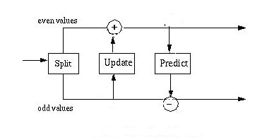
This modification of the lifting scheme places the update stage (which calculates the scaling function) before the predict stage. As before the predict stage is calculating the "predict" value from the smoothed values that result from the update stage. In this case the predict value is directly subtracted from the odd element. Another way to state this is that the result of the predict stage is a set of odd values that reflect the difference between an odd value and the 4-point polynomial interpolation result of the smoothed even values.
This algorithm is no longer a "pure" Lifting Scheme transform. The forward and inverse transform calculations of the update stage are not symetrical. The forward scaling function is

In the inverse transform, the inverse predict stage has returned the odd elements to their original values. The inverse scaling function is calculating by via the inverse of the average.
The result of the forward transform is shown below. Note that the absolute value of these wavelet coefficients is close to the range of the absolute value of the Haar transform coefficients.
A Haar scaling function combined with a polynomial interpolation wavelet function:
25.9375
-3.6875
8.3125 8.6875
-7.2344 10.2969 -2.0469 -28.0156
-15.8437 6.9688 -7.4062 4.8125 8.3125 -8.5625 -4.8125 6.4375
This wavelet algorithm is more accurate than the Haar transform, since it calculates the difference values over four points. This creates an overlap (as with the Daubechies D4 transform) that will properly capture change between odd and even values. This change is missed by the Haar transform.
A description of the Lifting Scheme version of the Daubechies D4 wavelet transform, along with Java source code, can be found on my Daubechies wavelet transform page.
Java implementations of the algorithms discussed on this page can be downloaded in the file lift.tar. This file archive contains the directories and files shown below.
lifttest.java
lifttest.cpp
C++/
C++/interp.h
C++/leastsq.h
C++/lifting.h
lift/
lift/daubechies.java
lift/haar.java
lift/haarpoly.java
lift/liftbase.java
lift/line.java
lift/poly.java
lift/polyinterp.java
The lift sub-directory contains Java implementions for the Haar, line and polynomial interpolation wavelets. These algorithms mirror the algorithms discussed on the predict wavelet web page.
The C++ directory contains a C++ version of the Haar transform extended with polynomial interpolation (e.g., lifting.h. This is supported by the interp.h class. The leastsq.h class is a C++ example of four point linear interpolation.
There is an associated Java package that contains some simple print routines (called util) which can be downloaded here (util.tar). This contains:
util/matrix.java
util/print.java
Most of the Java code that implements the wavelet software is packaged with an archive program called tar. The tar program is standard on UNIX, Linux and probably Mac OS X. Originally tar stood for tape archive. If you don't have a copy of tar for Windows NT you can download the win32 binary here. This version of tar is open source software, from Cygnus (now Red Hat), and came with the Cygwin32 package.
The material on this web page draws heavily from the book Ripples in Mathematics: The Discrete Wavelet Transform by A. Jensen and A. la Cour-Harbo, Springer, 2001. Obviously any errors here are mine. here.
Building Your Own Wavelets at Home by Wim Sweldens and Peter Schroder
Building Your Own Wavelets at Home is part of a course on Wavelets in Computer Graphics given at SigGraph 1994, 1995 and 1996.
The equations on this web page were created with the MathType program. MathType is a very easy to use program that allows the creation of equations that can then be output in GIF format. I used Microsoft's HTML Image Help editor to convert the GIF images to JPEGs.
Ian Kaplan
February 2002
Revised:
