Over the last year and a half or so I've been collecting wavelet books. One of these books is Essential Wavelets for Statistical Applications and Data Analysis by R. Todd Ogden. While I don't find that this book always provides the details I need to implement a particular wavelet technique, it does provide an interesting catalog of wavelet applications in statistics. One of these applications is histogram creation. I needed to create histogram plots for one of the web pages I've been writing, Wavelet compression, determinism and time series forecasting. So Ogden's discussion on using wavelets to create histograms was of immediate interest.
Early on in my wavelet adventures I wrote some histogram code in Java. I thought that wavelets might provide a more efficient method for generating histograms (as we shall see below, this does not seem to be the case). I was also fascinated by the idea that there was yet another application for wavelets (To a man with a hammer...). The only problem was that I did not fully understand Ogden's description.
Enlightenment did not arrive even after reading Ogden's description of wavelets applied to histograms a multiple times. Having failed with Ogden, I did what any modern person would do: I did a Web search using Google for wavelet histograms. Most of the references I found via Google were written by Min Wang or her colleagues or referenced their work.
Dr. Wang proposes using wavelet smoothed histograms for query optimization (for very readable discussion on query optimization see Chapter 16 of that most excellent of database books, Database Systems: the complete book by Garcia-Molina, Ullman and Widom). After reading Dr. Wangs papers and the first four chapters of her thesis and corresponding with her, I thought that I understood how to apply wavelet techniques for histogram creation.
A histogram is generated from a sample of values. The classic example is the height of each student in an introductory statistics class. The simple histogram algorithm that I've implemented here sorts these values and then divides them into histogram bins. The bins are created by dividing the value range by the number of bins (e.g., (maxValue - minValue)/numBins). This results in numBins bins, each of which covers an equal value range. Each bin will contain a count of the number of values in the data sample that fall within the range assigned to that bin. The number of values in a bin (the bin frequency) is usually plotted on the y-axis and the value range is plotted on the x-axis.
If the histogram is developed from integer values, the bins can simple be the integers between the minimum and maximum values.
In my histogram creation algorithm, the first step sorts the data. This has a time complexity of ONlog2N. When I first started reading about wavelets and histograms I hoped that somehow this sorting step could be avoided. Although there may be ways to avoid sorting, the wavelet transform does not have this advantage. So I'll assume that we start with the sorted data set shown below:
data set = {1, 2, 2, 2, 3, 3, 5, 5, 5, 5, 9, 9, 9, 10, 10, 12, 12, 13, 14}
The first step is to calculate the frequency of each value. This yields a pair of value/frequency pairs:
{vi, fi} = {1,1}, {2,3}, {3,2}, {5,4}, {9,3}, {10,2}, {12,2}, {13,1}, {14,1}
Plotting these pairs (with frequency on the y-axis and value on the x-axis) would yield an incorrect plot. There are intervening values which have zero frequency.
In step two, the frequency distribution is filled in for values with zero frequency.
In the data set above, the minimum value is 1 and the maximum value is 14. The value/frequency pairs with zero frequency filled in is shown below:
{vi, fi} = { 1,1}, { 2,3}, { 3,2}, { 4,0}, {5,4}, { 6,0}, { 7,0},
          { 8,0}, { 9,3}, {10,2}, {11,0}, {12,2}, {13,1}, {14,1}
Now if the value pairs are plotted we will see a histogram with correct frequency distribution, where the bin width is 1. This plot would be fine if there were only a few value/frequency pairs, as there are in this example. If there were many pairs, the plot would have a jagged edge. Histograms smooth this edge by grouping values into bins with a larger range.
The histogram can be smoothed using the wavelet transform. The wavelet transform is applied to data sets with a power of two values. The value/frequency set above can be converted into a data set with a power of two values (in this case, 16) by filling in extra values with zero frequency:
{vi, fi} = { 0,0}, { 1,1}, { 2,3}, { 3,2}, { 4,0}, {5,4}, { 6,0}, { 7,0},
          { 8,0}, { 9,3}, {10,2}, {11,0}, {12,2}, {13,1}, {14,1}, {15, 0}
In step three, the wavelet transform is calculated on the set of frequency values:
{fi} = {0}, {1}, {3}, {2}, {0}, {4}, {0}, {0},
       {0}, {3}, {2}, {0}, {2}, {1}, {1}, {0}
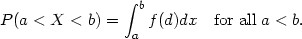
Figure 1 shows the result of the wavelet transform applied to sixteen values. The result of the transform consists of fifteen wavelet coefficients and an average value. The coefficients are ordered in bands of increasing frequency, where the band of eight coefficients at the right end of the array are the high frequency coefficients.
Figure 1
Step four sets selected wavelet coefficients to zero. For example, if the wavelet transform is applied to 512 frequency values, there will be wavelet coefficient bands with sizes 1, 2, 4, 8, 16, 32, 64, 128, 256. If the wavelet coefficient bands with sizes 64, 128 and 256 coefficient are set to zero, the histogram will be smoothed into 32 regions. This is not the same as 32 histogram bins, since the frequency in each region will remain the same.
A thresholding scheme can also be used to zero or modify wavelet coefficients. This is discussed in Min Wang's publications and in Noise Reduction by Wavelet Thresholding by Maarten Jansen (see references). Thresholding techniques may be useful if there is noise in the frequency distribution.
In step five the inverse wavelet transform is calculated. This will map the modified coefficient set into a data set for the smoothed histogram.
To support the analysis of financial time series data I need to calculate histograms over a floating point range (the frequency values remain integers). Unlike the integer histogram case, where the initial "bins" are defined by sequential integers, the bins in the floating point range must be explicitly calculated. The steps in applying the wavelet transform to calculate a histogram over a floating point range are outlined below:
Sort the data values.
Get the minimum and maximum values (e.g., v[0] and v[N-1]). Divide the range between the minimum and maximum values by a power of two (512, for example). This will be the bin size.
Distribute the values in the bins and calculate a set of bin/frequency values (e.g., {bin0,f0}, {bin1,f1}, ... {binN-1,fN-1})
The bins can be considered a numbered sequence from 0 to N-1, where each bin has an associated frequency (which may be zero). Calculate the wavelet transform on the frequencies array.
Set one or more high frequency wavelet coefficient bands to zero (or threshold the coefficients).
Calculate the inverse wavelet transform. The result will be a smoothed histogram.
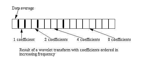
The close price for IBM over 513 trading days is shown below.
Figure 2
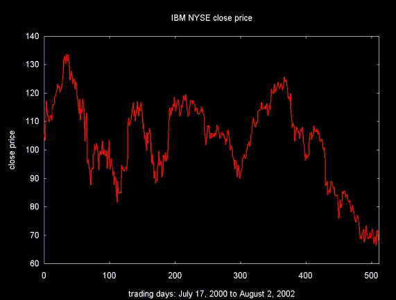
The 1-day return for a stock assumes that the stock is purchased one day and sold the next. In this case return is calculated as if there were no transaction costs (which is not the case in actual trading). The fractional 1-day return may be zero, positive or negative. The return is calculated as a fractional value of the original purchase price: (pt-1 - pt)/pt-1. Here t is time in trading days, pt-1 is yesterdays price and pt is today's price. Figure 3 plots 512 1-day fractional return values for IBM.
Figure 3
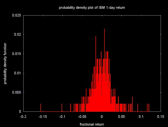
Figure 4 shows the distribution of the 512 value 1-day return time series (plotted in Figure 3) into 512 equal sized "bins".
Figure 4
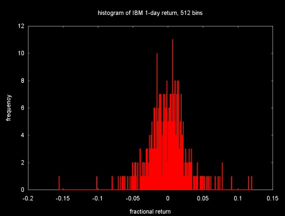
The frequencies obtained by dividing the fractional return values into histogram bins for a data set with 512 points. This data set can be used as the input for the wavelet transform (in this case, the normalized Haar wavelet transform). By setting selected high frequency wavelet coefficient bands to zero and inverting the wavelet transform, a smoothed version of the histogram can be obtained. This is shown in Figure 5, below. To generate this plot, the three highest frequency bands were set to zero (e.g., 64, 128 and 256).
Figure 5
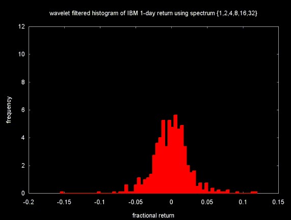
Figure 6 compares the smoothed histogram (plotted in white) to the original histogram (plotted in red).
Figure 6
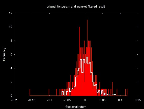
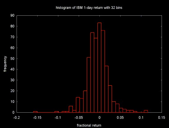
Figure 7 shows the original fractional return data set distributed into 32 histogram bins. Note that as the bin width spans a larger range, the frequence (the number of items that fall in a bin) also increases. This is not the case in the wavelet smoothed histogram.
Figure 7
Wavelet techniques applied to histograms can be considered a subset of density estimation in statistics. Density estimation is the calculation of a probability density function:
The probability density function is a fundamental concept in statistics. Consider any random quantity X that has probability density function f. Specifying the function f gives a natural description of the distribution of X, and allows probabilities associated with X to be found from the relation
From Density Estimation for Statistics and Data Analysis by B.W. Silverman, originally published in Monographs on Statistics and Applied Probability, Chapman and Hall, 1986. This book is published by CRC Press in the United States. The beginning of this book is republished on the Cal. Tech. web site.
If the bounds of the integral, a and b are the range of a given histogram bin, the probability density function is the probability that a given value will fall within the range of a given bin. This is simply calculated by dividing the frequency associated with a bin by the total frequency count. In the case of the histogram plotted in Figure 4, this is the frequency in a given bin, divided by 512.
Figure 8
A large sample of daily stock returns will fall into a Gaussian distribution. This is suggested by the examples above and is widely reported in the economics and finance literature. A Gaussian distribution can be described by the mean, the variance and other parameters (e.g., skew). These parameters can be plugged into the equation for a Gaussian curve to reconstruct the curve for the data.
This is logically similar to linear regression, where the line through a cloud of points is expressed by two constant parameters, a and b, in the equation y = ax + b.
Not all curves through a set of data points or data distributions can be described parametrically (with parameters like mean, variance, etc...). Non-parametric fits allow a function (e.g., a curve through points) to be estimated where simple parametric techniques would fail.
The probability density function in Figure 8 is obviously not smooth. This is the result of the fact that there are only 512 data samples. The probability density function will jump discontinuously from one bin to the next. Wavelets provide a way to do non-parametric smoothing of the probability density function, resulting in a smoother transition between one probability density function value and the next. This can be done by calculating the wavelet transform on the frequency or probability distribution, selectively modifying wavelet coefficients and calculating the inverse wavelet transform. For example, in wavelet thresholding, a threshold is calculated based on the wavelet coefficients. Coefficients are modified relative to this threshold value (see below).
There are an infinite variety of wavelet functions. The papers I've read on using wavelet histograms for query optimization use either the Haar wavelet or the linear interpolation wavelet. The papers on smoothing for density estimation use a variety of wavelet functions, including the Daubechies wavelets.
The wavelet library I have implemented in C++ (and Java) includes the Haar wavelet (in both normalized and unnormalized form), the linear interpolation wavelet and the Daubechies wavelet.
The equation used to calculate the threshold to use as a basis for altering wavelet coefficients is calculated from the standard deviation. Table 1 shows means and standard deviations for the wavelet coefficients calculated by the normalized Haar, linear interpolation and Daubechies D4 wavelet transforms applied to the 512 element 1-day return time series (note that the return histogram bins have not been converted into percentages, so these are not probability density function values). The mean and standard deviations are calculated for the four high frequency bands separately and for the bands together (e.g., coefficient elements 32 to 512).
| Norm. Haar | Linear Interp. | Daubechies D4 | ||||
|---|---|---|---|---|---|---|
| Band size | Mean | StdDev | Mean | StdDev | Mean | StdDev |
| 256 | 0.011049 | 1.009696 | 0.017578 | 1.165132 | -0.011049 | 1.021151 |
| 128 | -0.125000 | 1.062978 | -0.102539 | 1.199361 | 0.116066 | 1.113610 |
| 64 | 0.165728 | 1.180141 | 0.210449 | 1.339157 | -0.052427 | 1.116134 |
| 32 | 0.406250 | 1.046788 | 0.242432 | 0.812487 | -0.180837 | 0.624107 |
| 32 to 512 | 0.021740 | 1.055874 | 0.026253 | 1.181017 | 0.006012 | 1.038824 |
At least for this data set the mean and standard deviation for the Daubechies D4 coefficients is closest to a Gaussian normal distribution (e.g., mean = 0, stddev = 1). This distribution of the 1-day return is a Gaussian curve. Of the three wavelet functions, the Daubechies wavelet does the best in fitting the sine function (see the associated web page Spectral Analysis and Filtering with the Wavelet Transform). A half period sine wave is similar to the Gaussian curve, so I speculate that the Daucbechies D4 wavelet would be a good choice in this case as well.
Looked at from the lifting scheme point of view, the wavelet coefficients are the difference between the value "predicted" by the wavelet function and the actual data. If the wavelet function is a good match for the data, the wavelet coefficients will reflect noise in the data set. If this is the case, smoothing the data is the same as denoising. Wavelet denoising modifies a set of wavelet coefficients in reference to a threshold value. The inverse wavelet transform is then calculated to reconstruct the "denoised" signal.
Donoho and Johnstone describe a "universal threshold" (see Wavelet
Denoising References below)  :
:
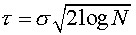
In this equation N is the number of wavelet coefficients that
are subject to thresholding and  is the standard deviation of the coefficients.
There are two basic methods in thresholding: "hard thresholding" and "soft thresholding":
In hard thresholding, any wavelet coefficient whose absolute value is less than the threshold value is set to zero. Coefficients whose absolute value is greater than or equal to the threshold are unchanged.
In the paper Nonlinear Wavelet Methods Donoho gives a modified version of the "universal threshold" for soft thresholding:
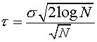
At least when it comes to smoothing the histogram/probability density function discussed on this web page, the modified universal threshold produces very poor results.
Other threshold values can be calculated on the basis of the Median Absolute Deviation of the wavelet coefficients (see the related web page Wavelet Noise Thresholding).
More complex adaptive thresholding algorithms have also been proposed. The most commonly used is the SURE algorithm (see papers by Donoho et al and the book by Jansen).
In section 10.5 of Percival and Walden (see book references, below) the threshold is calculated on only one coefficient band and then applied to all bands. Jansen calculates the threshold on all the coefficients. The approach I've followed is to calculate the threshold on the coefficients that are subject to modification. If only the four high frequency bands are thresholded, then the threshold is calculated on these bands. If all coefficients are thresholded, then the threshold is calculated on the entire coefficient set.
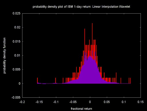
Figures 9, 10 and 11 show the the results of filtering the frequency histogram with the Haar, Daubechies D4 and linear interpolation wavelets. The threshold was calculated on wavelet coefficients 16 to 511 (as with C++, numbering is from 0). Soft thresholding is applied to the same range. After the coefficients are thresholded and the inverse transform is calculated, the frequency is converted to probability by dividing by the number of bins (512).
In all three Figures, the original probability density function is displayed in the background, in red. The filtered density function is shown in the foreground, in purple.
Figure 9 below shows the result of histogram smoothing using the Haar wavelet. After filtering, the blocky nature of the Haar wavelet produces a histogram like plot. Simply "re-binning" the histogram is much more computationally efficient.
Figure 9
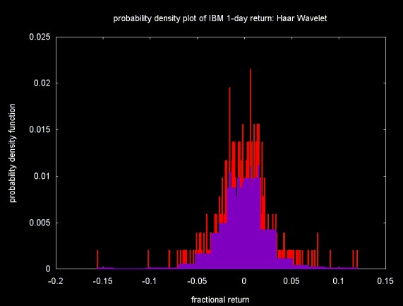
Figure 10 shows the result of the Daubechies D4 wavelet. The speculation above that the Daubechies D4 wavelet would produce the best fit for the underlying Gaussian distribution turns out to be incorrect. Although the Daubechies wavelet results in a smoother distribution than the Haar wavelet, the Daubechies wavelet introduces artifacts (these are more apparent in the original plot, which was larger).
Figure 10
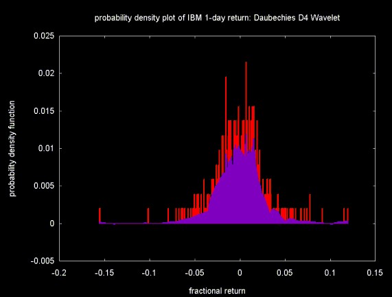
Figure 11 shows the result of the linear interpolation wavelet. The linear interpolation wavelet produces the smoothest distribution. At least for this example, the results are the best out of the three wavelet functions.
Figure 11
The distribution of 1-day returns contains spikes. One of the features of the wavelet transform and of wavelet thresholding is that it leaves large changes. These spikes can be seen all three figures above (although not clearly, since I've had to scale down the image sizes to avoid even higher download times). Whether this is desirable or not depends on the data and the application.
In many cases a data sample does not contain enough elements to fully resolve the distribution. There may be peaks and valleys that would not exist in a larger sample. By smoothing such a distribution, the shape that might exist for a larger sample can be uncovered. Smoothing also removes noise which may be present in the raw probability density function. Wavelets provide a useful technique for approximating the probability density function. Related work exists on using wavelets for non-linear, non-parametric regression.
Using wavelet techniques for simple histograms does not appear to be worthwhile, especially for floating point data. Applying wavelet techniques to a histogram of floating point data includes all of the computational effort needed to calculate the histogram, but also adds the computational overhead of the wavelet transform and, perhaps, thresholding. For many simple histograms, the smoothing properties of wavelets are unnecessary.
In studying wavelets applied to histograms I have learned a little about density estimation, which has been interesting (and potentially useful). Especially when it comes to removing noise from a density estimation, wavelets may provide a useful tool.
The C++ software to calculate histograms, the wavelet transforms, and the soft threshold, along with the a small equity data set, can be downloaded here. This file is in UNIX tar format and is compressed with gzip (GNU Zip). The "tar" file includes the stock close price data displayed here, along with the code to read these data sets.
If you are using a Windows system and you don't have tar and gzip you can down load them by clicking on the links below. This code is courtesy of Cygnus (now Red Hat) and is Free Software.
I am grateful to Dr. Min Wang at the IBM Watson Research Center (and previously Duke University) who was kind enough to answer my e-mail questions about the application of wavelets to histogram creation. Dr. Wang's application of wavelets to database query optimization is much more sophisticated than the simple creation of histograms, discussed here.
The work of Professor Gilbert G. Walter of the University of Wisconsin on wavelets applied to histograms and density estimation has been referenced by a number of authors, including Todd Ogden (see below). Professor Walter was kind enough to answer my questions on wavelet techniques applied to histograms and density estimation.
None of the people I have corresponded with are responsible for the contents of this web page. Any errors are mine.
Essential Wavelets for Statistical Applications and Data Analysis by R. Todd Ogden, Birkhäuser, 1997
This book discusses histogram creation using wavelets. I found the description very difficult to follow, which lead me to the references below (which were not easy, but I eventually did make progress).
I find this book a useful outline for wavelet applications. However, the applications are outlined largely using mathematical equations, with few lucid examples. I sometimes wonder if anyone can actually develop applications based on this kind of material. But perhaps this is simply a reflection of my modest mathematical skills.
Noise Reduction by Wavelet Thresholding by Maarten Jansen, 2001, Springer Verlag Lecture Notes in Statistics, No. 161
Wavelet Methods for Time Series Analysis by Percival and Walden, Cambridge Univ. Press, 2000
Chapter 10 covers Wavelet-Based Signal Estimation. Section
10.5 discusses threshold calculation based on the Median Absolute
Deviation. This was the reference I used for my earlier web page Wavelet
Noise Thresholding. Percival and Walden also discuss the
"universal threshold" equation, however, they use variance (e.g.,  ), instead of standard deviation. Percival and Walden
are math Gods, so it's likely that I'm missing something here. But
there interpretation of the universal threshold seems to me to be
different from Donoho's.
), instead of standard deviation. Percival and Walden
are math Gods, so it's likely that I'm missing something here. But
there interpretation of the universal threshold seems to me to be
different from Donoho's.
The papers by Min Wang and her thesis advisor, Prof. Vitter at Duke University are some of the most most influential references on histograms and wavelets. These papers deal with wavelet generated histograms applied to database query optimization. This is also the topic of Dr. Wang's Phd thesis. The application discussed in these papers goes beyond simple histogram creation.
These references are all available from Dr. Min Wang's web site at Duke University (at the time of this writing, Dr. Wang was a Research Staff Member at IBM's T.J. Watson Research Center.
Approximation and Learning Techniques in Database Systems by Min Wang, Phd Thesis, Department of Computer Science Duke University, 1999
Dr. Wang's Phd thesis discusses calculation of wavelet histograms for data base applications.
Dynamic Maintenance of Wavelet-Based Histograms by Y. Matias, J. S. Vitter and M. Wang, September 2000
Wavelet-Based Histograms for Selectivity Estimation Y. Matias, J. S. Vitter and Min Wang, Proceedings of the 1998 ACM SIGMOD International Conference on Management of Data (SIGMOD '98), Seattle, Washington, June 1998, 448-459.
Fast Wavelet Histogram Techniques for Image Indexing by M. K. Mandal, and T. Aboulnasr
Wavelet generated histograms are used as indices (keys) for image search and retrieval.
Efficient Time Series Matching by Wavelets, by Kin-pong Chan and Ada Wai-chee Fu, 1999
This paper has nothing to do with histograms generated using wavelet techniques. I've included it here as a bookmark for future reference. This paper was referenced in Wavelets and their Applications in Databases (below). The paper outlines a method for using wavelet techniques to fetch time series data on the basis of a similarity measure with another time series or on a subsequence key.
Wavelet Shrinkage and W.V.D.: A 10-Minute Tour by David L. Donoho, 1993
The PDF for this paper is damaged on Prof. Donoho web site at Stanford (at least as far as my Acrobat reader is concerned). The NEC version is readable.
Nonlinear Wavelet Methods for the Recovery of Signals, Densities, and Spectra from Indirect and Noisy Data, David L. Donoho, 1993, in PDF format
Density estimation by wavelet thresholding by David L. Donoho, Iain M. Johnstone, Gerard Kerkyacharian, and Dominique Picard, April 1993
Warning: this paper is mostly mathematics. I found it pretty much unreadable.
Wavelets and their Applications in Databases by Daniel Keim and Martin Heczko (in PDF format).
This is a beautifully put together set of slides from a talk on wavelet applications. These slides provide an interesting overview of many wavelet applications. There are some excellent slides on database (referencing the work of M. Wang et al above) and data mining applications.
Approximate Query Processing: Taming the TeraBytes! A Tutorial by Minos Garofalakis and Phillip B. Gibbons
This tutorial was given at the 2001 International Conference on Very Large Databases. The tutorial provides some nice outlines for the work that M. Wang et al did no applying wavelets in database query optimization.
The slides were originally created using Microsoft Power Point. The link above is a PDF translation of the power point slides. I don't know how permanent this link will be. Minos Garofalakis currently has a web page at Lucent's Bell Labs.
Ian Kaplan
September 2002
Revised:
Back to Wavelets and Signal Processing