My interest in wavelets began with the idea that the wavelet transform could be used to filter out noise. The idea behind noise filtering is to remove the noise while leaving the important detail. While this is fine as an ideal, it is hard to realize in practice.
Wavelets do provide a powerful way to analyze non-stationary time series (e.g., time series were the Fourier transform is not successful). While there is a great deal of material on wavelets, there is less accessable material on wavelets and noise filtering. The definition of noise turns out to be somewhat arbitrary. If we come up with a definition of noise, how do we prove that it applies to the time series we are interested in? Here I've decided that the noise in an equity close price time series is gaussian. If we were dealing with intra-day bid/ask prices I'd lean more toward Poisson noise.
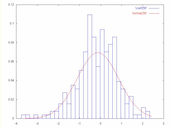
The histogram plot of the highest frequency Haar coefficients suggests that the theory that there is gaussian noise in the close price time series may be reasonable. The mean is close to zero and the standard deviation is close to one. The histogram is shown along with a Gaussian or normal curve with the same mean and standard deviation.
Highest frequency coefficient spectrum: points 256 to 511
The histogram plots on this Web page were generated by the bell_curves class in the wavelet_util package published with the wavelet java code.
The highest frequency coefficients are proportional to the change in the close price between two successive days. This is also proportional to the daily return, which financial theory states is normally distributed.
One technique that has been proposed for filtering wavelet coefficients is to zero the coefficients that are within an error range of the mean. However, this may remove important information. In the case of the histogram above, there are points outside the curve which may represent meaningful movement in the time series.
The idea behind the gaussian filter used here is that every point that falls within a gaussian curve is balanced by another point on the other side of the curve. So it is the points that lie outside the curve that may show important movement in the time series. If the gaussian curve is subtracted from the histogram, we will be left with those points that are outside the curve.
As the coefficient spectrum frequency decreases we see larger detail in the time series. The first graph shows price movement over a two day period. The graph below shows price movement over a four day period. As the frequency decreases the mean moves farther away from zero and the standard deviation increases.
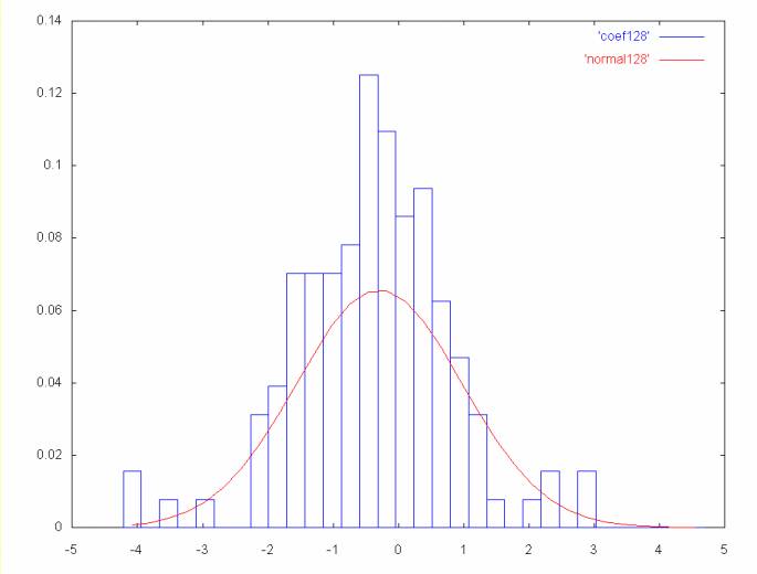
Coefficient spectrum points 128 to 255
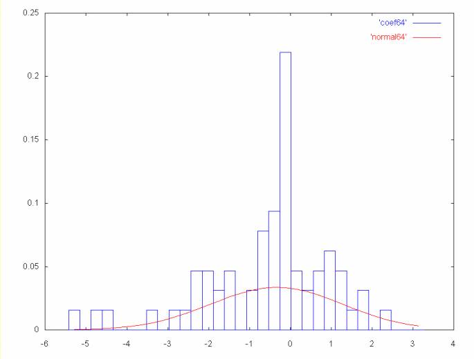
Coefficient spectrum points 64 to 127
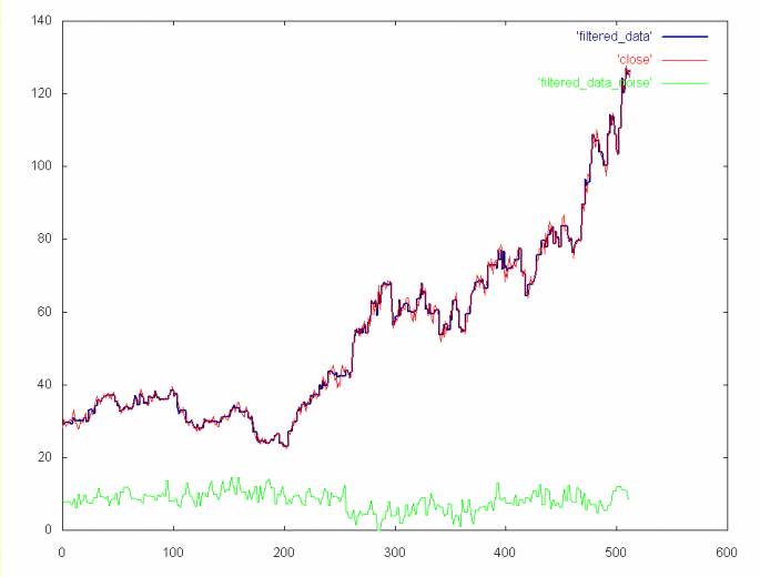
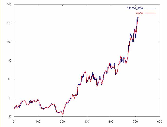
When the Gaussian curve is subtracted from the histogram in the case of the AMAT close price time series, 311 points (or about 60 percent) are set to zero. When the inverse Haar transform is applied we get the time series shown below.
The ideal in filtering is to remove noise while leaving important detail. The graph below compares the wavelet noise filter to a cubic spline applied to the AMAT close price time series. The cubic spline leaves out much of the detail compared to the Gaussian noise filter.
This noise filtering algorithm is expensive, since the Gaussian curve is numerically integrated over the range of each histogram bin. On top of this there is the overhead of calculating the histogram, which is O(n log2n). If we were filtering thousands of equity time series, this might prove to be too computationally expensive. However, this does demonstrate the power of data filtering using wavelet techniques.
Not only is the curve subtraction expensive, but in the case of the AMAT time series it is only marginally better than the the time series with the noise spectrum removed (see the plot of the time series without the 256 spectrum shown here).
Ian Kaplan, July 2001
Revised:
back to Applying the Haar Wavelet Transform to Time Series Information
