A power spectrum can be calculated from the result of a wavelet transform. Plotting the power spectrum provides a useful graphical representation for analyzing wavelet functions and for defining filters.
This web page views the wavelet transform largely in the frequency domain. The wavelet transform can also be used for time/frequency analysis, which is covered on the related web page Frequency Analysis Using the Wavelet Packet Transform.
A wavelet function can be viewed as a high pass filter, which aproximates a data set (a signal or time series). The result of the wavelet function is the difference between value calculated by the wavelet function and the actual data. The scaling function calculates a smoothed version of the data, which becomes the input for the next iteration of the wavelet function. In the context of filtering, an ideal wavelet/scaling function pair would exactly split the spectrum. For example, if the sampled frequency range is 0 to 1024 Hz, the result of the wavelet function would be signals from 512 to 1025 Hz. The result of the scaling function would be signals from 0 to 511.
There are an infinite variety of wavelet and wavelet scaling functions. The closeness of the approximation provided by the wavelet function depends on the nature of the data. How closely the wavelet and scaling functions approach ideal filters depends on the nature of these functions and how they interact with the data.
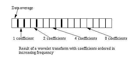
Figure 1, below shows the logical structure of the result of a wavelet transform calculated on a 16-element data set. The element labeled "data average" is the result of the final application of the scaling function. In the case of the Haar wavelet function, this will be the average of the data set. Following the data average are the wavelet coefficient bands, whose size is an increasing power of two (e.g., 20, 21, 22...)
Figure 1
If the data set consists of N elements, where N is a power of two, there will be log2(N) coefficient bands and one scaling value. For example, in the case of the 16 element wavelet result diagrammed in Figure 1, there are four bands (log2(16) = 4). The wavelet power spectrum is calculated by summing the squares of the coefficient values for each band.
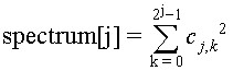
In the spectrum plots below the average is squared as well. This results in the square of the average at spectrum0 and the square of the first coefficient band at spectrum1.
Software download
The C++ software for the wavelet functions, the signal generation and the spectrum calculation can be downloaded here. This file is in UNIX tar format and is compressed with gzip (GNU Zip). The "tar" file includes the stock close price data displayed here, along with the code to read these data sets.
If you are using a Windows system and you don't have tar and gzip you can down load them by clicking on the links below. This code is courtesy of Cygnus (now Red Hat) and is Free Software.
Doxygen Generated Documentation
The doxygen generated documentation for this software can be viewed here
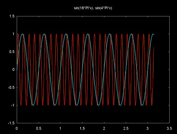
A stationary data set is a data set where the sample can be viewed as repeating infinitely if the data set were also infinitely extended. An example of a stationary data set is a data set composed of sine and/or cosine waves. Figure 2 shows two sine waves, 16*Pi*x and 4*Pi*x in the region 0..Pi.
Figure 2
The data set plotted in Figure 3 is the result of summing the two sine waves shown in Figure 2. The components that make up this signal are well separated in terms of frequency. Applying the Fourier transform would clearly show the signal components (for example, see Figure 10 in Frequency Analysis Using the Wavlet Packet Transform). Since the Fourier transform works well on such a data set, it makes a good comparision for wavelet spectral analysis.
Figure 3
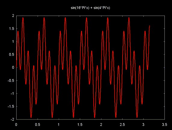
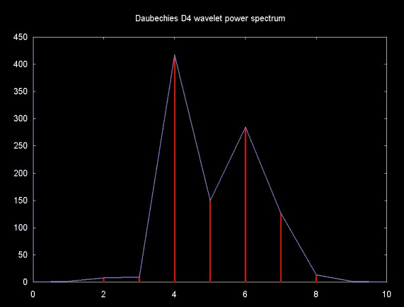
Figure 4 shows the wavelet power spectrum for the result of the Daubechies D4 transform applied to the signal shown in Figure 3, sampled at 1024 points. The point plotted at zero on the x-axis is the square of the single scaling function value that is left after calculating the wavelet transform. The wavelet coefficient bands are plotted at x-axis points 1 to 10. These correspond to bands with 20 to 29 coefficients (e.g., 1, 2, 4,... 512). The wavelet coefficient band farthest out on the x-axis (plotted at x-axis point 10) contains differences between the wavelet function and the signal. The better the approximation provided by the wavelet function the smaller these values will be. The Daubechies D4 wavelet provides a reasonably good approximation since both bands 9 and 10 have small values. The Daubechies D4 wavelet is also able to localize both of the signal components, as shown by the two peaks in the power spectrum plot.
Figure 4
Selected parts of the spectrum localized by the wavelet transform can be isolated by selectively copying wavelet coefficient bands into a new vector and calculating the inverse wavelet traansform. The first element in the wavelet transform result, the scaling value, is always copied, since it is needed to reconstruct the data using the inverse transform. The parts of the wavelet transform that are not copied are set to zero.
Using the wavelet power spectrum in Figure 4 as a guide, an attempt can be made to reconstruct the two signals that make up the signal shown in Figure 3. A low pass filter is created by copying the scaling value and wavelet coefficient bands 1 ... 5. A high pass filter is created by copying bands 6 ... 10. All values outside of these bands will be set to zero. The inverse wavelet transform is then calculated on each of these vectors. Figure 5 shows the result. The low pass filter (wavelet coefficient bands 1 ... 5) is shown in red. The high pass filter (wavelet coefficient bands 6 ... 10) is shown in blue.
The reconstruction of the component signals is not perfect, although the frequency in both cases is correct. The cycles of the lower frequency signal are no longer shaped like sine wave cycles but like the Daubechies wavelet function.
Figure 5

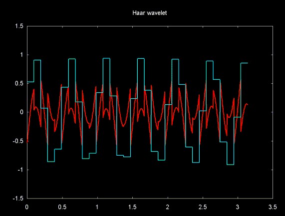
The square basis for the Haar wavelet does an even worse job of approximating sine waves, as the artifacts in Figure 6 show. As in Figure 5, Figure 6 shows two signals reconstructed from the coefficient bands 1 ... 5 (shown in blue) and 6 ... 10 (shown in red).
Figure 6
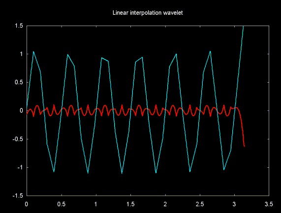
Like the Haar wavelet, the linear interpolation wavelet captures the low frequency component, but does poorly with the high frequency component.
Figure 7
The ability of a wavelet filter to exactly reconstruct a signal component depends on how closely the wavelet function approximates the signal. To demonstrate this, the linear interpolation wavelet is applied to a sawtooth wave.
The linear interpolation wavelet function predicts that an odd element will be located on a line between two even elements. The linear interpolation scaling function calculates the average of the even and odd elements. Since the linear interpolation wavelet is a sloped line, it can exactly approximate the sawtooth wave.
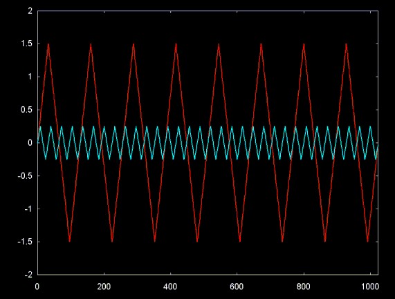
Figure 8 shows two sawtooth waves: a low frequency 8-cycle wave and a higher frequency 32-cycle wave.
Figure 8
The signal in figure 9 shows the sum of the two signals in figure 8, sampled at 1024 points.
Figure 9
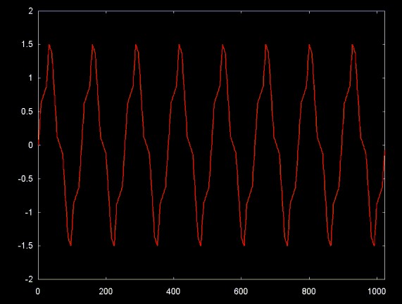
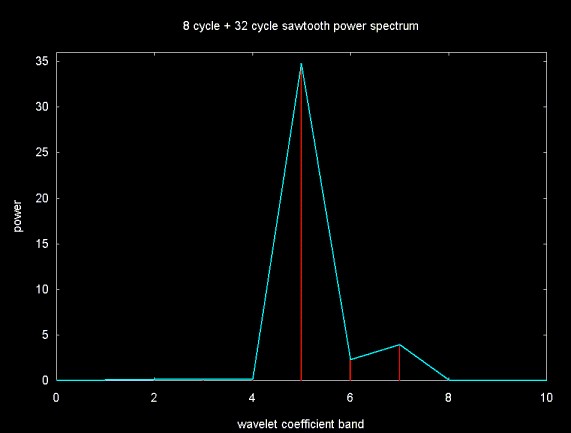
Figure 10 shows the power spectrum for the result of the linear interpolation wavelet transform. Note that bands 9 and 10 are zero (or close to zero), since the linear interpolation wavelet has closely approximated the sawtooth signal. The two sub-components can be seen peaking in bands 5 and 7.
Figure 10
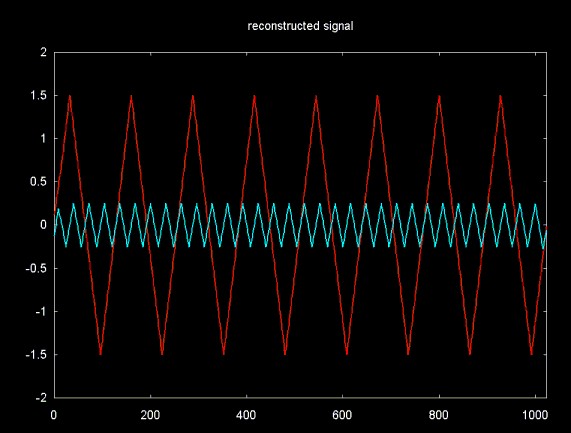
A low pass filter is created by copying bands 1 ... 6 and a high pass filter is created by copying bands 7 ... 10. The inverse wavelet transform is then applied to each vector, resulting in the signals shown in Figure 11. Note that the linear interpolation wavelet almost exactly reconstructs the original signal.
Figure 11
As the sawtooth example above shows, the ability of a wavelet function to decompose a signal into its component parts depends on how closely the wavelet approximates the data set. A wavelet basis function based on a circle would be expected to do an excellent job in filtering signals composed of sine and cosine waves. A wavelet based on a single sine wave cycle would predict that a signal element lay on the sine wave basis and store the difference. While the wavelet function can be clearly envisioned, the scaling functions is not as obvious. The ideal scaling function paired with the proposed sine basis wavelet should be a complementary low pass filter which divides the sampled spectrum. The calculation of a scaling function for an arbitrary wavelet function is not obvious, at least to me.
Plotting the power spectrum of the result of the wavelet transform allows us to analyze how well (or poorly) the wavelet function resolves the signal components. The power spectrum of the polynomial interpolation wavelet transform applied to the signal in Figure 3 is shown on the associated web page Spectral Analysis and Filtering with a Polynomial Interpolation Wavelet. This is an example where the wavelet function is poorly matched with the signal. In fact, the power spectrum plot suggests that this polynomial interpolation wavelet may not be a good choice for any application.
My original motivation for studying wavelets was inspired by the idea of denoising stock market time series data (e.g., daily and intra-day stock market data). See Applying the Haar Wavelet Transform to Time Series Information. The examples that follow apply spectral analysis of the linear interpolation wavelet to time series composed of stock market close prices downloaded from finance.yahoo.com. Financial time series are similar to the sawtooth wave discussed above, so it can be expected that the linear interpolation wavelet is a good choice.
The existence of stationarity in stock market time series (e.g., market behavior that repeats in a cyclical manner) seems to be a matter of faith on both the pro and con side. There are those who believe in market cycles like Elliot waves. There is a remarkable vanity documentary that was made by a very successful trader named Paul Tudor Jones, where he and a colleague are enthusiastically pointing to Elliot wave plots. Mr. Jones' success speaks for itself, but I don't think that it is based on finding cycles in the market. I do not believe that such cycles exist in the equities market. But proving a negative is difficult and it certainly has not been shown that market cycles don't exist. So disbelief in market cycles is based somewhat on faith as well.
the point of this digression on market cycles is that by using wavelet tecniques I am not trying to find underlying cycles. My interest is in filtering the data or extracting other information (for example, a measure of determinism).
In this discussion, I separate cyclical stationarity from determinism. As Andrew Lo et al point out in their book A Non-Random Walk Down Wall Street there is structure in the stock market, especially short term structure. Wavelet techniques may helpful in uncovering some of this structure.
Figure 12 shows the close price for Applied Materials, a company that makes semiconductor fabrication equipment. The time series consist of market close prices for a period of slightly less than two years (e.g., 512 trading days). All the data used here was downloaded from finance.yahoo.com.
Figure 12
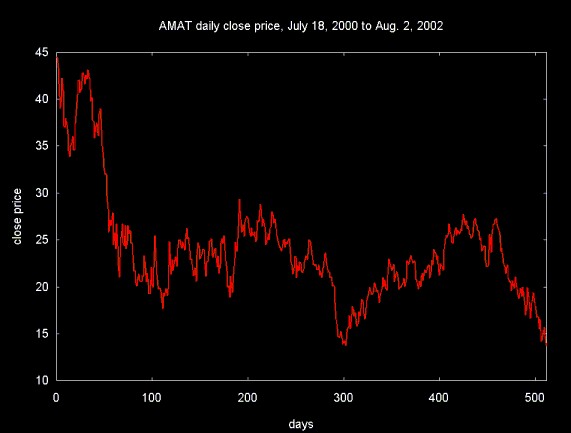
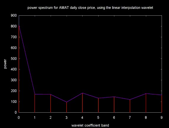
Figure 13 shows the power spectrum of the result of the linear interpolation wavelet transform. The absence of obvious cyclical components in this time series is reflected in the power spectrum, which is approximately flat.
Figure 13
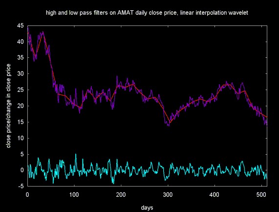
Two filters are created, a low pass filter from bands 1 ... 5 and a high pass filter from bands 6 ... 9. The result of the inverse linear interpolation wavelet applied to these bands is shown in Figure 14. The low pass filter is plotted in red. The close price which this filter approximates is plotted in purple. The result of the high pass filter is plotted in blue-green.
Figure 14
The power spectrum for the result of the linear interpolation wavelet applied to a time series composed of 512 close prices for IBM is shown in figure 15. It shows slightly more structure than the power spectrum for AMAT, but it is still approximately flat.
Figure 15
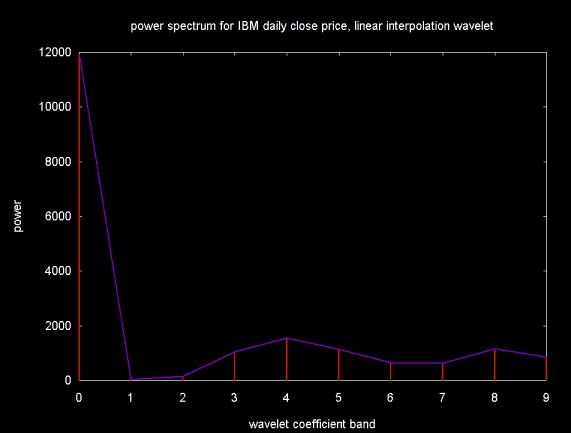
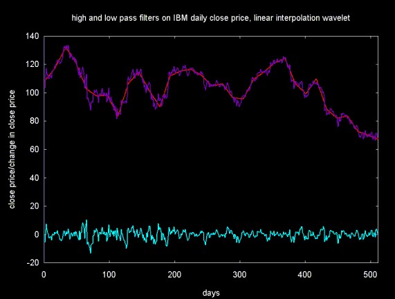
Figure 16 shows low and high pass filters constructed from wavelet coefficient bands 1 ... 5 and 6 ... 9, respectively.
Figure 16
Financial models are frequently based on returns, rather than directly on market data (e.g., open or close prices). In the examples that follow, wavelet filters are applied to a time series coposed on 1-day returns.
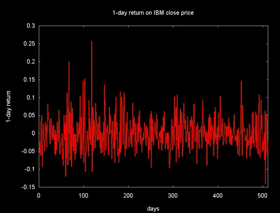
The economics literature reports that daily returns are distributed in a Gaussian curve, centered around zero. This is certainly suggested by the 1-day return time series for IBM shown below. The one day return is calculated by (vi-1 - vi)/vi-1, where v is the close price for IBM on a given day.
Figure 17
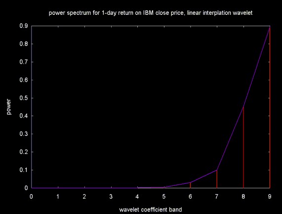
The power spectrum for the return series is poorly approximated by the linear interpolation wavelet. Figure 18 shows a peak in wavelet coefficient band 9, which is the initial difference between the value predicted by the linear interplation wavelet and the return series.
Figure 18
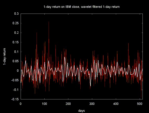
From its appearance, the return series contains significant amounts of noise. Low pass filters can be used to remove noise (although they may also remove signal as well). The result of a low pass filter (in white) plotted with the return series (in red) is shown in Figure 19. The low pass filter is created by copying wavelet coefficient bands 1 ... 7.
Figure 19
Forecasting via Wavelet Scalograms: theory and application by Miguel A. Arinno
Dr. Arinno (there is a tilda over the n, which I am approximating in english with "nn") kindly mailed me this paper, along with several others describing his work using wavelet filters as an aid in time series prediction. I did not understand wavelet power spectrum plots (also referred to as scalograms) until I read this paper. I had one of those "ah ha" moments reading this paper and immediately started writing the software and generating the plots that serve as the basis for this web page.
Ripples in Mathematics: the Discrete Wavelet Transform by Arne Jense and Anders la Cour-Harbo, Springer, 2001
This book has been the core reference for my later work on wavelets.
Trading Volume-Conditions Relationships Between Past Return, Contemporaneous Return and Future Return by Adam Y.C. Lei, Louisiana State University, Sept. 4, 2001
This articles discusses short term market structure based on return.
The plots displayed on this web page were generated with GnuPlot. Equations were created using MathType.
Ian Kaplan
August 2002
Revised:
Back to Wavelets and Signal Processing
