The wavelet transform is commonly used in the time domain. For example, wavelet noise filters are constructed by calculating the wavelet transform for a signal and then applying an algorithm that determines which wavelet coefficients should be modified (usually by being set to zero). (Wavelet coefficients are the result of the high pass filter applied to the signal or to combinations of low pass filters of the signal.) Although these coefficients are associated with frequency components, they are modified in the time domain (each coefficient, ci, corresponds to a time range).
In contrast to the wavelet transform, the Fourier transform takes a signal in the time domain (e.g., a signal sampled at some frequency) and transforms it into the frequency domain, where the Fourier transform result represents the frequency components of the signal. Once the signal is transformed into the frequency domain, we lose all information about time, only frequency remains.
What would be nice is a a signal analysis tool that has the frequency resolution power of the Fourier transform and the time resolution power of the wavelet transform. To some extent the wavelet packet transform gives us this tool. I write "to some extent" because as this web pages shows, the wavelet packet transform does not produce as exact a result as the Fourier transform and the wavelet packet result is more difficult to interpret. The wavelet packet transform can be applied to time varying signals, where the simple Fourier transform does not produce a useful result.
Wavelets and digital signal processing are topics that are too complex to cover easily in a set of web pages, or even in a single book (as my growing library of wavelet and DSP references attests). The contribution that I see these web pages making is the publication of C++ and Java code that implements these algorithms. I also have tried to provide some material that explains these algorithms. But it is obvious to me that my explanation is incomplete and is best read along with a more detailed explanation, which covers some of the mathematical background. I recommend Ripples in Mathematics: the Discrete Wavelet Transform by Jensen and la Cour-Harbo, Springer Verlag, 2001. The material on this web page relies heavily on Chapter 9 of Ripples. Any mistakes on this web page are mine.
The C++ code that builds the frequency ordered wavelet packet tree extends the standard wavelet packet code and is published with this code in a single tar file (see The Wavelet Packet Transform).
The C++ source code for the wavelet packet/frequency ordered wavelet packet algorithms can be downloaded here.
The doxygen generated documentation for this code can be found here
This web page builds on the related web page The Wavelet Packet Transform (which covers material in Chapter 8 of Ripples in Mathematics). The result of the wavelet packet transform is not ordered by increasing frequency. By result, I am referring to the "level basis", which is a horizontal slice through the wavelet packet tree. If each node in the level basis is numbered with a sequential binary grey code value (0000, 0001, 0011, 0010, 0110,...) the nodes can be ordered by frequency by sorting them into decimal order (0001, 0010, 0011,...) I regard this as a mathematical curiosity, since the wavelet packet transform can be calculated in frequency order by proper ordering of the low and high pass filters.
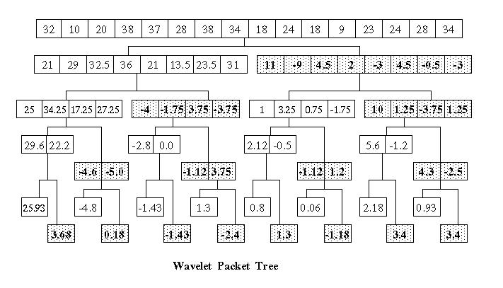
In the standard wavelet packet transform the result of the scaling function (the low pass filter) is placed in the lower half of the array and the result of the wavelet function (the high pass filter) is placed in the upper half of the array. The wavelet packet algorithm recursively applies the wavelet transform to the high and low pass result at each level, generating two new filter results which have half the number of elements. The standard transform is shown in figure 1. The result of the wavelet (high pass) filter is shaded.
Figure 1
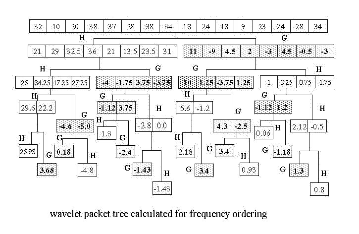
If we think of the lower and upper halves of the array that results from the wavelet transform as two children in the wavelet packet tree, a frequency ordered wavelet packet result can be calculated inverting the location of the filter results in the left hand child. This is shown in Figure 2. In this diagram the low pass filter is shown as H and the high pass filter is shown as G. The high pass filter results are shaded as well.
The first wavelet trasform produces the result
  left child  = H1 = {21, 29, 32.5, 36, 21, 13.5, 23.5, 31}
  right child = G1 = {11, -9, 4.5, 2, -3, 4.5, -0.5, -3}
The standard wavelet transform is applied to the left child (e.g., the result of the low pass filter H is placed in the lower half o the result array and the result of the high pass filter G is placed in the upper half of the array.
A modified wavelet transform is applied to the right child. Here the result of the high pass filter G is placed in the lower half of the array and the result of the low pass filter H is placed in the upper half of the array.
Each recursive step generates two more children, where the standard transform is applied to the left child and the modified transform is applied to the left child.
Figure 2
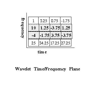
The best time/frequency resolution is obtained by taking a level basis through the tree which results in a square matrix. For the wavelet packet tree this in Figure 2 this is a matrix composed from the four element element arrays that result from the second application of the wavelet transform. The tree is walked from left to right. If the maximum frequency is f, the first array will contain the frequency range {0 .. (f/4)-1}, the second array will contain frequencies {f/4 .. (f/2)-1}, the third array will contain frequencies {f/2 .. (3/4 *f)-1} and the four array will contain {3/4*f .. f }. On the time axis there are four time steps.
As Figure 3 shows, these arrays are stacked to form a matrix, where the x-axis is time and the y-axis is frequency. This is shown below in Figure 3.
Figure 3
As the time/frequency plots on this web page demonstrate, the modified version of the wavelet packet transform does indeed produce a frequency orders result. The fact that this is the case is not immediately obvious.
Let us assume that the wavelet transform is a perfect filter and that we have a signal that ranges from {0..64Hz). The low pass scaling function (H) results in exactly the lower half of the frequency spectrum {0..32Hz} and the high pass wavelet function results in exactly the upper half of the spectrum {32..64Hz}. After the first transform step, the low pass result is on the left branch of the tree and the high pass result is on the right branch. The usual filter pair (H, G) is applied to the right branch and the inverse filter pair (G, H) is applied to the right branch. As the modified wavelet packet tree is recursively built this way, it is not obvious that the result is frequency ordered.
Both Ripples in Mathematics and Wavelet Methods for Time Series Analysis (see the references at the end of the page) spend several pages explaining how frequency ordering works in the wavelet packet transform. So far I have not found a shorter way to explain this. My intent in writing these web pages is not to replace references like Ripples in Mathematics but to expand on the material covered in these references. So I'm going to "punt" on this issue and refer the reader to Chapter 9 of Ripples in Mathematics and Chapter 6 of Wavelet Methods for Time Series Analysis (for those who are more mathematically "hard core", as the Marines would say if they were mathematicians). For the purposes of this web page I'll ask the reader to "stipulate" (as the lawyers suing Enron would say) that the result of the modified wavelet packet transform shown in Figure 2 is frequency ordered.
A square matrix constructed from a level basis can be used to build a three dimensional plot, where the z-axis is a function of the value at m[y][x]. Many authors use a grey scale plot to represent the z-axis values (e.g., an x-y plot where the z-dimension is the shade of grey. Math and statistics environments like Matlab and S+ support grey scale plots. Although I have access to these packages at work, this material is developed with my own computer resources, so I have used 3-D surface plots rendered with gnuPlot.
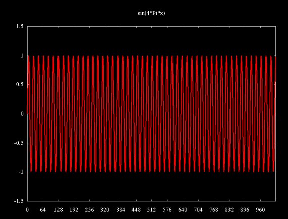
The power of the wavelet transform is that it allows signal variation through time to be examined. Frequently the first example used for wavelet packet time/frequency analysis is the so called linear chirp, which exponentially increases in frequency over time. Rather than jumping into the linear chirp, let us first look at a simple sine function. Figure 4 shows the function sin(4Pix), in the range {0..8Pi}, sampled at 1024 evenly spaced points.
Figure 4
A magnitude plot of the result of a Fourier transform of the sampled signal is shown in Figure 5 (here only the relevant part of the plot is shown). This shows a signal of about 51 cycles, which is what I get when I count the cycles by hand. The data for this discrete Fourier transform (DFT) plot was calculated using Java code which can be found here.
Figure 5
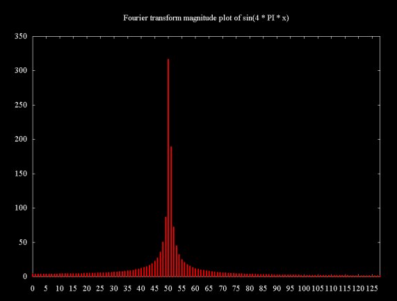
The Fourier transform plots on this web page do not show adjusted magnitude (where adjMag = 2Mag/N), so the magnitudes do not properly represent the signal magnitude.
Figure 6a shows a frequency/time plot using wavelet packet frequency analysis. As with the examples above, this plot samples the signal sin(4Pix) in the range {0..8Pi} at 1024 equally spaced points. A square 32x32 matrix is constructed from 32 elements arrays from the fifth level of the modified wavelet packet transform tree (where we count from zero, starting at the top level of the tree, which is the original signal). Frequency is plotted on the x-axis and time on the y-axis. The z-axis plots the founction log(1+s[i]2). A gradient map is also shown on the x-y plane.
Figure 6(a)
Why are there peaks in this plot? The peaks are formed by the filtered signal at the resolution of the level basis. Since the z-axis plots log(1+s[i]2), the part of the sine wave that would be below the plane is flipped up above the plane.
The wavelet frequency/time plot in 6(a) is not as easy to interpret as the Fourier transform magnitude plot. The signal region is shown in Figure 6(b), scaled to show the signal region in more detail.
Figure 6(b)
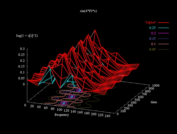
The wavelet signal is spread out through a range of about 80 cycles, centered at slightly over 100. The Fourier transform of sin(4x) shows that there are 51 cycles in the sample. Is the wavelet packet transform reporting a value that is double the value reported by the Fourier transformm? I don't know the answer. The wavelet packet transform has been developed in the last decade. Where books like Richard Lyons' Understanding Digital Signal Processing cover Fourier based frequency analysis in detail, this depth is lacking the the literature I've seen on the wavelet packet transform.
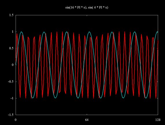
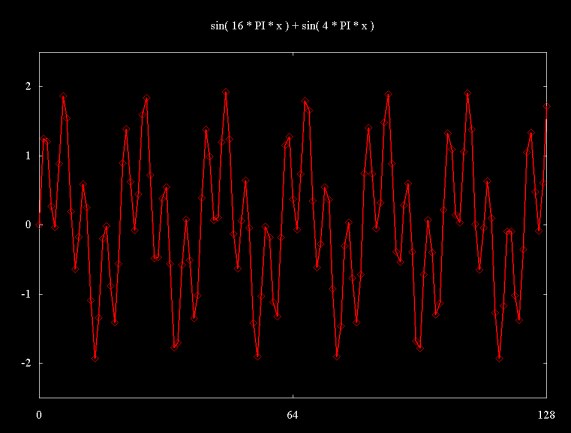
The Fourier transform is a powerful tool for decomposing a signal that is composed of the sum of sine (or cosine) waves. The plot below super imposes two sine waves, sin(16Pix) and sin(4Pix).
Figure 7
When these two signals are added together we get the signal show below in Figure 8 (shown in detail)
Figure 8
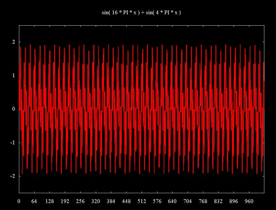
The same signal, plotted through a range of {0..32Pi} and sampled at 1024 equally spaced points is shown below.
Figure 9
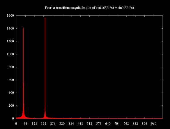
The Fourier transform result in Figure 10 shows that this signal is composed the 51 cycle sin(4Pix) signal and another signal of about 200 cycles (sin(16Pix)). This is a case where the Fourier transform really shines as a signal analysis tool. The two signal components are widely spaced, allowing clear resolution.
Figure 10
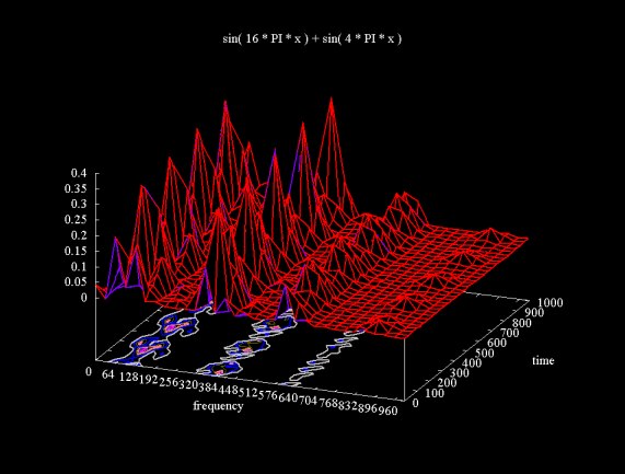
The wavelet packet transform plotted in Figure 11 shows two signal components, the sin(4Pix) component we saw in Figures 6(a) and 6(b) and the higher frequency component from sin(16Pix). Again, the wavelet packet transform result is not entirely clear. As the Fourier transform result shows, the higher frequency signal component is about four times the frequency of the lower frequency component. This is not quite the case with the wavelet packet transform, where the second frequency component appears to be slightly less than four times the frequency of the sin(4Pix) component. The surface plot also shows two echo artifacts at higher frequencies.
Figure 11
For stationary signals that repeat through infinity, where the signal components are sufficiently separated, the Fourier transform can clearly separate the signal components. However, the Fourier transform result is only in the frequency domain. The time component ceases to exist. Also, the basic Fourier tranform does not provide very useful answers for signals that vary through time. Figure 12 shows a plot of a sine wave where the frequency increases by Pi/2 in each of eight steps.
Figure 12
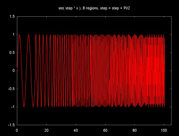
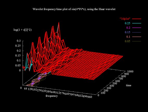
Figure 13 (a) shows a surface plot of the modified wavelet packet transform applied to this signal (using the Haar wavelet). The surface ridge shows the increasing frequency, although the steps cannot be clearly isolated, perhaps because the frequency difference between the steps is not sufficiently large. The ridges above 512 on the frequency spectrum are artifacts.
Figure 13 (a)
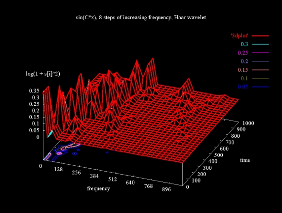
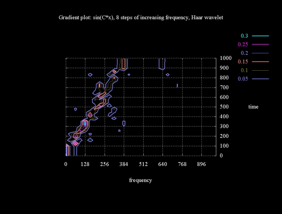
Figure 13 (b) shows a gradient plot, using the same data as Figure 13 (a). As with the surface plot representation, we can see the frequency increase, but the step wise nature of this increase cannot be seen.
Figure 13 (b)
The modified wavelet packet transform is frequently demonstrated using a "linear chirp" signal. This is a signal with an exponentially increasing frequency, calculated from the equation:
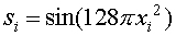
Figure 14 shows a plot of the linear chirp signal in the region {0..2}, sampled at 1024 points. As the linear chirp frequency increases, the signal becomes undersampled, which accounts for the jagged arrowhead shape of the signal around 0 as xi gets closer to 2.
Figure 14
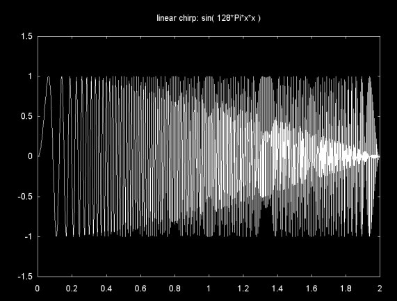
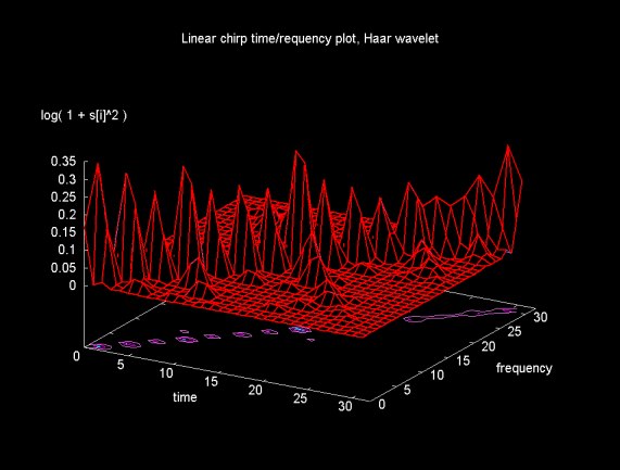
Figure 15 shows the result of the modified wavelet packet transform, using the Haar wavelet, applied to the linear chirp. The peaks exist because the signal is sampled at a particular resolution and the absolute value of the signal is plotted. Note that as the frequency increases the peaks seem to disappear as the signal cycles get close together.
The ridge along the diagonal shows that the signal frequency increases through time. In theory the linear chirp frequency increases exponentially, not linearly as this plot suggests. However, the signal is sampled at a finite number of points, so the exponential nature of the signal disappears as the signal becomes under sampled. The ridges that are perpendicular to the main diagonal line are artifacts.
Figure 15
In theory the Daubechies D4 wavelet transform (e.g., four scaling (H) and four wavelet coefficients (G)) is closer that the Haar wavelet transform to a perfect filter that exactly divides the frequency spectrum. The closer the (H, G) filters are to an ideal filter, the fewer the artifacts in the wavelet packet transform result. The result of applying the modified wavelet packet transform, using Daubechies D4 filters, to the linear chirp is shown in figure 16.
Figure 16
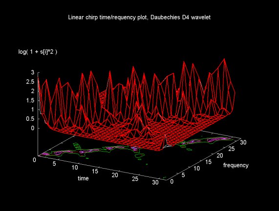
The result in Figure 16 is certainly not better than that obtained using the Haar transform and, in fact, may be worse. In Ripples in Mathematics, the authors give an example of wavelet packet transform results using Daubechies D12 filters. There are notable fewer artifacts in this case. Jensen and la Cour-Harbo mention that as the filter length approaches the signal size, the filter approaches an ideal filter.
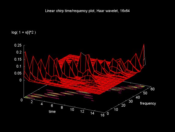
The plots in Figures 15 and 16 come from 32x32 matrices (where the original sample consisted of 1024 points). Time is divided up into 32 regions (as is frequency). Can we get better time/frequency resolution by decreasing the range of the time regions and increasing the number of frequency regions?
Figure 17 shows a surface plot of a 16x64 matrix generated from the next "linear basis" (e.g., a horizontal slice through the wavelet packet tree at the next level). As the gradient plot on the x-y plane shows, the time frequency localization is not improved.
Figure 17
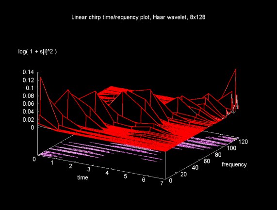
The plot in Figure 18 is generated from an 8x128 matrix. By further reducing the time regions, all the frequency bands become compressed into a smaller time region. Multiple frequency bands become associated with a given time region.
Figure 18
The modified wavelet packet transform gives us a tool that can be used to analyze time varying signals. Although this tool can be used in cases where the simple Fourier transform does not provide good results (either because a time/frequency answer is needed or because the signal varies through time), the wavelet packet transform is more difficult to use and understand. On this web page, the wavelet packet transform has been examined using only two wavelets: Haar and Daubechies D4. Other wavelets can produce better answers. All the examples here use a "level basis". A non-level bases can be chosen using a cost function (Shannon entropy, as discussed on this related web page). A non-level basis is even more difficult to interpret (not to mention plot) since it is composed of several time/frequency regions from the wavelet packet tree.
In short, this web page is hardly the last word on using the wavelet packet transform for time/frequency analysis. At most this web page provides some examples drawn from a complex topic. I suspect that if I understood wavelet filter bank theory better some of the issues of time/frequency localization would become clearer.
Ripples in Mathematics by Jensen and la Cour-Harbo, Springer Verlag, 2001
As noted in the acknowledgements section above, this is the primary reference I have used to learn to use the modified wavelet packet transform for time/frequency analysis.
Wavelet Methods for Time Series Analysis by Percival and Walden, Cambridge University Press, 2000
Wavelet Methods for Time Series Analysis is a much more mathematically intensive text on wavelets and wavelet methods, including the wavelet packet transform and the modified wavelet packet transform discussed on this web page. When I can't find an answer (or understand an answer) to a question about wavelets, I've used this book.
This web page discusses the standard wavelet packet transform on with the frequency ordered transform discussed here is based. This web page also discusses the calculation of the "best basis", which is a minimal representation of the data set relative to a particular cost function.
Wavelets and Signal Processing
This is the main "table of contents" page for the material I've written on wavelets and signal processing. This includes a link to some material I wrote on the Fourier transform and the Java code that was used to generate the Fourier transform data shown on this page.
Ripples in Mathematics web page.
This is the web page by the authors of Ripples in Mathematics. It includes links to a number of sub-pages, including pages that publish Matlab and C source code for the algorithms discussed in the book.
Ian Kaplan
May 2002
Revised:
Back to Wavelets and Signal Processing
