Lossless Wavelet Compression
Introduction
This web page discusses lossless data compression using integer to
integer wavelet transforms and an integer version of the wavelet
packet transform.
The lossless compression discussed here involves 1-D data. However,
these algorithms directly generalize to 2-D data (e.g., images) [1].
Applications for lossless compression include compression of
experimental data and compression of financial time series (for
example, the bid/ask time series that arise from intra-day trading).
Usually a technique like integer to integer wavelet compression is
applied to a large data set (like an image) as the first step in the
compression process. A second data coding step is applied. Ideally
the first step will result in repeated value (either sequential
repeats or multiple occurrences of a given value), so additional
compression can be achieved by a coding algorithm like Huffman or run
length coding.
The motivation behind this web page is not data compression per
se. Wavelet compression is a form of predictive compression.
Predictive compression algorithms can be used to estimate the amount
of noise in the data set, relative to the predictive function.
Turning this around, wavelet compression, especially wavelet packet
compression can be used to estimate the amount of determinism in a data
set. This can be useful in time series forecasting, since a region
with low noise and high determinism may be a region that is more
predictable. In terms of wavelet compression, a region that is
relatively compressible may be more predictable. This web page lays
the foundation for the related web page Wavelet
compression, determinism and time series forecasting. The example
time series used here are stock market close prices for a small set of
large capitalization stocks.
Along with this discussion on lossless wavelet compression, I have
published the C++ source code for these algorithms.
format).
Data Compression
Data that is compressed via a lossless compression algorithm can
exactly recovered by the decompression algorithm. Lossless
compression algorithms are used to compress data where loss cannot be
tolerated. For example, text, experimental data or compiled object
code. The lossless compression program gzip (GNU Zip),
a Free Software compression program, is widely used on UNIX and
GNU/Linux systems for lossless compression.
Lossy compression algorithms are not perfectly invertible. The
decompressed result of a lossy compression algorithm is an
approximation of the orignal data. Lossy compression algorithms are
frequently used to compress images and digitized sound files.
Computer display and sound playback devices have limited resolution. The
human eye and ear are also limited in their resolution. In many cases
selected image and sound data can be removed without reducing the
perceived quality of the result.
One notable exception to lossy image compression is medical images.
While selected data can be removed from these images without
observable loss of quality, no one wants to take the chance of
removing detail that may be important. Medical images are frequently
transmitted using lossless compression.
This web page and the algorithms published here concentrate on 1-D
financial time series data (e.g., stock market close price). These
compression algorithms will generalize directly to 2-D data. In many
2-D image compression algorithms, the first step of the compression
algorithm converts the 2-D image data into a linear vector. For
example, a 1,024 x 1,024 pixel image can be converted to linear form
by linearizing the rows of the image to create a vector of 1,048,576
pixel elements (see [1]
for an excellent discussion of image linearization).
The data sets used as examples here are small relative to image and
sound files. A wavelet compression algorithm applied to a large data
file would be followed by a coding compression step, like Huffman or
run length coding. Such a coding step is of little use for a small
data set, since the result of the compression algorithm frequently has
few repeat values.
Data Compression and Determinism
Data compression is a fascinating topic when considered by itself.
This web page examines lossless data compression as a method to
estimate the amount of determinism, relative to noise, in a financial
time series. Estimating the amount of determinism (or noise content)
in a signal region may be useful in time series forecasting. This is
discussed on the related Web page Wavelet
compression, determinism and time series forecasting.
Deterministic data is generated by some underlying process which is
not entirely random. For example, the water level of the Nile river
is influenced by the seasonal rains, which provide an underlying
deterministic process. The water level on any given day is influenced
by daily rain, which is a random event. This creates a time series
for the Nile river water level that consists of deterministic
information mixed with random information, or noise.
If a magic compression algorithm existed that could exactly model all
deterministic processes, the data left after these deterministic
values were subtracted would be noise (data generated by a
non-deterministic process). Given a starting set of values, our magic
compression function would be able to predict all the deterministic
values in the data set. So given the value s0 the
magic compression function could calculate all of the other values
s1 to sn. If there was no noise
in the deterministic data the magic compression algorithm could
compress the data set to a small set of values, consisting of the
initial starting state and the length of the data set to be generated.
At the other end of the spectrum, is a data set this is composed
entirely of values generated by a non-deterministic process (e.g.,
noise). This data set cannot be compressed to any significant degree.
Cellular automata, fractal functions, the calculation of pi to
N places and pseudo-random number generators are examples of functions
that can generate extremely complex results from a simple starting
point. There is no magic compression function that will discover the
function and starting value for given a data sequence. In practice, a
compression algorithm uses, at most, a small set of approximation
functions. This function is used to "predict" values in the data set
from earlier values. For example, we might chose a linear compression
function that predicts that the value si+1 will be
equal to si. The difference between this prediction
function and the data set is the incompressible information. This is
the Lifting Scheme version of the Haar wavelet transform. Another
compression function might be chosen which predicts that the point
si lies on a line running between the points
si-1 and si+1. The difference
between the predicted value at si and the actual
value at si is the incompressible data. This is the
linear interpolation wavelet. Other prediction functions include
4-point polynomial interpolation and spline interpolation.
In wavelet terminology, the predictive function is referred to as the
wavelet function. The wavelet function is paired with a scaling
function. The wavelet function acts as a high pass filter. The
scaling function acts as a low pass filter, which avoids aliasing
(large jumps in data values).
Most modern compression techniques use a two step process:
-
A predictive compression function (perhaps a wavelet transform) is
applied in the first step. If the predictive compression function is
a good fit for the data set, the result will be a new data set with
smaller values, and more repetition.
-
A coding compression step that attempts to represent the data set in
its minimal form. A coding compression algorithm like Huffman coding
is applied to the result of the predictive step. Ideally the
predictive step will result in smaller values, with some values that
are repeated.
Predictive compression yields good results for image compression,
where the change from pixel to pixel is not an entirely random process
(assuming that the image is of something other than random noise). A
predictive step would be useless for text compression however, since
there is no underlying deterministic process in a natural language
text stream that can be approximated with a function. Text
compression relies on data representation compression (coding
compression).
If we have a compression program, it would be nice if there was a
metric that would tell us how efficient our compression program is.
The Shannon entropy equation is frequently referenced in the
compression literature. What can Shannon entropy equation tell us?
Integer to Integer Wavelet Transforms
The wavelet transform takes an input data set and maps it to a
transformed data set. When a floating point wavelet transform is
applied to an integer data set, the transform maps the integer data
into a real data set. For example, an integer data set S is
shown below.
S = {32, 10, 20, 38, 37, 28, 38, 34, 18, 24, 18, 9, 23, 24, 28, 34}
When the Lifting Scheme version of the Haar transform is applied to
the data set, the integer data set is mapped to the set of real
numbers shown below.
25.9375
-7.375
9.25 10.0
8.0 3.5 -7.5 7.5
-22.0 18.0 -9.0 -4.0 6.0 -9.0 1.0 6.0
If the input data set is not random and a wavelet function is chosen
that can approximate the data on one or more scales, the wavelet
transform will produce a result that represents the original data set
as a set of small values, with a few large values that are of the
magnitude of the original data. This is a round about way of stating
that the original data set has been compressed using a predictive
compression algorithm.
The object of a compression algorithm is to represent the original
data in fewer bits. If the wavelet transform maps an integer data set
into a floating point data set, no compression may have been achieved,
since the fractional digits must be represented. In fact,
a set of floating point results may require more bits
than were needed to represent the original integer data set.
If the compression algorithm is lossy, the result of the wavelet
transform can be rounded to integer values or small values may be set
to zero. By modifying the result of the wavelet transform, perfect
invertibility is lost and the original input data can not be exactly
regenerated. A lossy compression algorithm might be appropriate for
the image compression used for Web page images, but it would be
totally unacceptable for compressing the data from a chemistry
experiment or a financial time series. Lossy compression also does
not provide as good an estimate for calculating the amount of
deterministic information in a time series, since some information has
been discarded.
Integer to integer wavelet transforms map an integer data set into
another integer data set. These transform are perfectly invertible
and yield exactly the original data set. An excellent discussion of
integer to integer wavelet transforms can be found in [2],
particularly sections 3 and 4. This web page relies heavily on this
paper (of course any mistakes are mine).
Any wavelet transform can be generalized to an integer to integer
wavelet transform. For example in [2] an
integer to integer version of the Daubechies D4 wavelet transform is
presented.
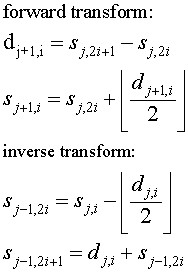
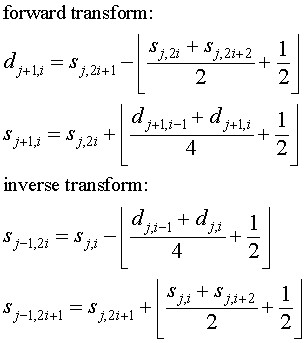
I have implemented three integer to integer Lifting Scheme wavelet
transforms. This are listed below, along with the equations for the
forward and inverse transform. One of the elegant things about the
wavelet Lifting Scheme is that the inverse transform is the mirror of
the forward transform, with the + and - operators
interchanged.
-
An integer version of the Lifting Scheme version of the Haar
transform. In image processing this is known as the S transform.
-
An integer version of the linear interpolation wavelet transform. The
linear interpolation transform "predicts" that an odd element will be
on a line between its two even neighbors. The difference between this
"prediction" and the actual value becomes the wavelet coefficient
(sometimes called the detail coefficient). The scaling function is
simply the average of the original even and odd elements.
-
An integer version of the Cohen-Daubechies-Feauveau (3,1) wavelet
transform. This is sometimes referred to as the TS transform in the
image processing literature.
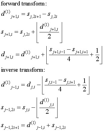
The wavelet lifting scheme is discussed on the related web page Basic Lifting
Scheme Wavelets. The equations above correspond to lifting scheme
steps.
The notation used here is based on the notation in [2],
so I'll briefly try to explain it.
The forward wavelet transform takes N elements in step j and
calculates N/2 detail coefficients (shown as d above)
and N/2 scaled values (shown as s above). The scaled
values become the input for the next step of the wavelet transform
(which is why these values are shown with the subscript j+1).
In the next step, Nj+1 = Nj/2.
The inverse wavelet transform in step j rebuilds the
sj-1,i and sj-1,i+1 (even and odd elements) from
the dj and sj values.
Compression and Small Data Sets
Compression is usually applied to large data sets. The estimation of
the power of the compression algorithm is based on the number of bits
needed to represent the compressed data set.
Compared to media data, like images, sound or video, the amount of
data in a time series that we are trying to develop a forecast (for
example, these "close" price for a stock) is
relatively small. The window of data that the compression algorithm
is applied to in forecasting may be even smaller.
A coding step (for example, Huffman coding or the Variable Bit Length
Coding proposed in [2])
applied to the result of the predictive step attempts to represent the
data in a minimal number of bits. The coding step can find a more
compact representation for the data when there are long runs of values
(say 28) that can be represented in the same number of bits
or when the frequency distribution of values is not uniform.
The wavelet result for a relatively small data set (say 64 or 128
values) will tend to have few repeat values (e.g., a frequency close
to 1/N for each value, in the case of N values). Huffman and other
"dictionary" based coding schemes work poorly in this case. Since the
data set is relatively small, there may not be large runs of values
that can be represented in the same number of bits.
The motivation for the work discussed here is to use compression (the
number of bits needed to represent the data set after the transform)
to estimate the amount determinism in the data set. If a high degree
of compression is achieved then the wavelet algorithm closely
approximated the original data set, leaving only small residual
values. This indicates that there was a high degree of determinism,
relative to the wavelet function.
Rather than applying a classic compression coding scheme to estimate
the number of bits needed to represent the wavelet result, a simple
total for the number of bits is calculated. The total number of bits
needed for to represent the wavelet result is the sum of the bit
widths for each element. For a real compression algorithm, where the
result must be decompressed as well, this represents an impractical
lower bound. In a real compression algorithm a sub-sequence of values
would be allocated in a common number of bits per value. A header for
the subsequence, perhaps with a count and a width indicator would
proceed the sequence. These headers and the common value widths
in a sequence increase the size of the compression result.
Results
This section discusses the results of applying wavelet algorithms to a
set of stock close price time series. In all cases these time series
consist of 512 elements. The data was down-loaded from Yahoo. This data is in
"decimalized" form (e.g., there are only two fractional decimal
digits, representing US cents). The fixed point data is multiplied by
100 to convert it to integer form. The list of stocks is shown below,
in Table 1.
Table 1
| NYSE/NASDQ Symbol |
Company |
| aa | Alcoa Aluminium |
| amat | Applied Materials |
| ba | Boeing |
| cof | Capital One |
| ge | General Electric |
| ibm | IBM Corp. |
| intc | Intel |
| mmm | 3M Corp |
| mrk | Merck |
| wmt | Wal-Mart |
The three integer to integer wavelet algorithms discussed above (Haar,
linear interpolation and the TS transform) were applied to the data
sets. An integer version of the wavelet packet transform, using the
linear interpolation wavelet, was also used. The cost function for
the wavelet packet transform was bit width.
To provide a comparison for the more complex wavelet algorithms, a
simple difference compression algorithm was also applied (I refer to
this as "delta"). A data set of N elements is replaced by the
differences. In this simple algorithm
si = si - si-1.
For an array indexed from 0, i = 1 to N-1. The element at
s0 is the reference element, which is unchanged. The next
element at s1 is replaced by the difference between that
element and s0.
The "delta" algorithm is very simple and has a time complexity of N,
where as the wavelet algorithm is Nlog2N.
Table 2 shows the results of the compression algorithms. The values
are the total number of bits needed to represent the data set. This
total is an impractical lower bound arrived at by adding up the number
of bits needed to represent each element. While this lower bound is
not practical for a real compression algorithm, it does provide a
reasonable metric for comparing the results.
Table 2, Compression for 512 element data sets
| Symbol |
Uncompressed |
delta |
Haar |
line |
TS |
wavelet packet (line) |
| aa | 7188 | 4071 | 4291 | 4155 |
4134 | 3876 |
| amat | 7059 | 4199 | 4415 |
4214 | 4272 | 3966 |
| ba | 7572 | 4279 | 4467 | 4320 | 4302 | 4118 |
| cof | 7664 | 4603 | 4824 | 4571 | 4696 | 4368 |
| ge | 7423 | 4146 | 4341 | 4155 | 4210 | 3977 |
| ibm | 8140 | 4829 | 5013 | 4826 | 4842 | 4627 |
| intc | 7211 | 4355 | 4555 | 4379 | 4400 | 4115 |
| mmm | 8188 | 4592 | 4807 | 4613 | 4688 | 4479 |
| mrk | 7728 | 4315 | 4512 | 4273 | 4319 | 4144 |
| wmt | 7680 | 4285 | 4474 | 4213 | 4276 | 4030 |
The data for this table was generated by the compresstest.cpp
code in the lossless/src subdirectory in the source code
directory tree.
Discussion
One surprising result is that the simple "delta" compression algorithm
compares very well to the slower, more complicated wavelet
algorithms, in terms of compression. In fact, in several cases the
"delta" algorithm yields better results. Another interesting result
is that in all cases the integer version of the wavelet packet
algorithm yields the best result.
The wavelet packet algorithm yields a "best basis" set, where sections
of the data set are represented by wavelet functions at different
scales. The scale chosen is the scale that minimizes the cost
function (in this case bit width). Another way to view this is that
the wavelet packet function provides the best approximation for the
data, relative to a given wavelet function.
The wavelet packet algorithm is also the slowest algorithm. Like all
wavelet algorithms, it's time complexity is 0Nlog(N).
However, the O factor will be bigger for the wavelet packet
algorithm because of its more complicated data structure. The wavelet
packet data structure must also be traversed by the cost function and
the best basis function, which selects the best basis set.
The code needed to implement the wavelet packet algorithm is also
larger, so it has a higher Kolmogorov complexity than either the
simple "delta" algorithm or a standard wavelet algorithm.
Although the wavelet packet function is not without its extra cost, it
is a better choice for estimating the determinism in a time series,
since it provides a close fit for the data. In short term time series
forecasting the wavelet packet algorithm would be applied to
relatively small windows of data. The computational cost of the
integer to integer wavelet packet algorithm is not so high that it
could not be used in real time on a modern high speed processor.
C++ Source Code and Documentation
The integer to integer wavelet transforms and the integer version of
the wavelet packet transform reuses some of the software implemented
for floating point wavelet transforms and the floating point wavelet
packet algorithm. As a result, this software is included in the
lossless subdirectory in source code for wavelet packets. A
data subdirectory includes the test data sets (historical
stock close prices down-loaded from Yahoo). The data
subdirectory also include the yahooTS class which reads these
data sets from disk.
The C++ source code for wavelet packets and lossless wavelet
compression algorithms can be down-loaded from this
web page.
The doxygen generated documentation can be found here
References (Books)
-
A Guide to Data Compression Methods by David Solomon, Springer
Verlag, 2002
-
Ripples in Mathematics by Jensen and la Cour-Harbo, Springer
Verlag, 2001
-
An Introduction to Kolmogorov Complexity and Its Applications
by Ming Li and Paul Vitanyi, Second Edition, Springer Verlag, 1997
This book has been a pleasant surprise. The book is carefully written
and understandable with a basic background in discrete math. The
authors take great care to explain the notation they use and they
write clearly. The book is dense with ideas (and mathematics), which
makes it a time consuming read. I have a theory that fully
understanding a book like this may take the reader as long as it took
the authors to write the book.
-
State of the Art
Lossless Image Compression Algorithms by S. Sahni, B.C. Vemuri,
F. Chen, C. Kapoor, C. Leonard, and J. Fitzsimmons, October 30, 1997
-
Wavelet Transforms
that Map Integers to Integers by A.R. Calderbank, Ingrid
Daugbechies, Wim Sweldens, and Boon-Lock Yeo, 1996
Ian Kaplan
August 2002
Revised:
Back
to Wavelets and Signal Processing
