|
|||||||||
| PREV CLASS NEXT CLASS | FRAMES NO FRAMES | ||||||||
| SUMMARY: INNER | FIELD | CONSTR | METHOD | DETAIL: FIELD | CONSTR | METHOD | ||||||||
java.lang.Object
  |
  +--wavelet_util.plot
        |
        +--wavelet_util.bell_curves
class bell_curves
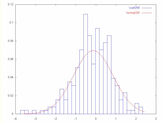
Plot the Haar coefficients as a histogram, in Gnuplot format. In another file generate a normal curve with the mean and standard deviation of the histogram. Using two files allows the histogram and the normal curve to be plotted together using gnu plot, where the histogram and normal curve will be different colored lines. If the spectrum as 256 coefficient points, the files generated would be coef256 and normal256 for the coefficient histogram and the normal curve. To plot these using gnuplot the following command would be used:
plot 'coef256' with boxes, 'normal256' with lines
This will result in a gnuplot graph where the histogram is one color and the normal curve is another.
A normal curve is a probability distribution, where the values are plotted on the x-axis and the probability of that value occuring is plotted on the y-axis. To plot the coefficient histogram in the same terms, the percentage of the total points is represented for each histogram bin. This is the same as the integral of the normal curve in the histogram range, if the coefficient histogram fell in a perfect normal distribution. For example;
| Inner Class Summary | |
private class |
bell_curves.bell_info
Bell curve info: mean, sigma (the standard deviation) |
private class |
bell_curves.bin
A histogram "bin" |
private class |
bell_curves.low_high
Encapsulate the low and high values of a number range |
| Constructor Summary | |
bell_curves()
|
|
| Method Summary | |
(package private) java.lang.String |
class_name()
|
private void |
histogram_coef(java.io.PrintWriter prStr,
               int num_bins,
               bell_curves.low_high m,
               double[] v)
Write out a histogram for the Haar coefficient frequency spectrum in gnuplot format. |
private void |
normal_curve(java.io.PrintWriter prStr,
             int num_bins,
             bell_curves.low_high m,
             double[] v)
Output a gnuplot formatted histogram of the area under a normal curve through the range m.low to m.high based on the mean and standard deviation of the values in the array v. |
private double |
normal_interval(bell_curves.bell_info info,
                double low,
                double high,
                int num_points)
normal_interval |
void |
plot_curves(double[] coef)
This function is passed an ordered set of Haar wavelet coefficients. |
private void |
plot_freq(double[] v)
plot_freq |
bell_curves.bell_info |
stddev(double[] v)
Calculate the mean and standard deviation. |
| Methods inherited from class wavelet_util.plot |
OpenFile |
| Methods inherited from class java.lang.Object |
|
| Constructor Detail |
public bell_curves()
| Method Detail |
java.lang.String class_name()
public bell_curves.bell_info stddev(double[] v)
Calculate the mean and standard deviation.
The stddev function is passed an array of numbers. It returns the mean, standard deviation in the bell_info object.
private double normal_interval(bell_curves.bell_info info,
                               double low,
                               double high,
                               int num_points)
normal_interval
Numerically integreate the normal curve with mean info.mean and standard deviation info.sigma over the range low to high.
There normal curve equation that is integrated is:
f(y) = (1/(s * sqrt(2 * pi)) e-(1/(2 * s2)(y-u)2
Where u is the mean and s is the standard deviation.
The area under the section of this curve from low to high is returned as the function result.
The normal curve equation results in a curve expressed as a probability distribution, where probabilities are expressed as values greater than zero and less than one. The total area under a normal curve is one.
The integral is calculated in a dumb fashion (e.g., we're not using anything fancy like simpson's rule). The area in the interval xi to xi+1 is
area = (xi+1 - xi) * g(xi)
Where the function g(xi) is the point on the normal curve probability distribution at xi.
info - This object encapsulates the mean and standard deviationlow - Start of the integralhigh - End of the integralnum_points - Number of points to calculate (should be even)
private void normal_curve(java.io.PrintWriter prStr,
                          int num_bins,
                          bell_curves.low_high m,
                          double[] v)
Output a gnuplot formatted histogram of the area under a normal curve through the range m.low to m.high based on the mean and standard deviation of the values in the array v. The number of bins used in the histogram is num_bins
prStr - PrintWriter object for output filenum_bins - Number of histogram binsm - An object encapsulating the high and low values of vv - An array of doubles from which the mean and standard deviation is calculated.
private void histogram_coef(java.io.PrintWriter prStr,
                            int num_bins,
                            bell_curves.low_high m,
                            double[] v)
Write out a histogram for the Haar coefficient frequency spectrum in gnuplot format.
prStr - PrintWriter object for output filenum_bins - Number of histogram binsm - An object encapsulating the high and low values from vv - The array of doubles to histogram
private void plot_freq(double[] v)
                throws java.io.IOException
plot_freq
Generate histograms for a set of coefficients (passed in the argument v). Generate a seperate histogram for a normal curve. Both histograms have the same number of bins and the same scale.
The histograms are written to separate files in gnuplot format. Different files are needed (as far as I can tell) to allow different colored lines for the coefficient histogram and the normal plot. The file name reflects the number of points in the coefficient spectrum.
public void plot_curves(double[] coef)
This function is passed an ordered set of Haar wavelet coefficients. For each frequency of coefficients a graph will be generated, in gnuplot format, that plots the ordered Haar coefficients as a histogram. A gaussian (normal) curve with the same mean and standard deviation will also be plotted for comparision.
The histogram for the coefficients is generated by counting the number of coefficients that fall within a particular bin range and then dividing by the total number of coefficients. This results in a histogram where all bins add up to one (or to put it another way, a curve whose area is one).
The standard formula for a normal curve results in a curve showing the probability profile. To convert this curve to the same scale as the coefficient histogram, the area under the curve is integrated over the range of each bin (corresponding to the coefficient histogram bins). The area under the normal curve is one, resulting in the same scale.
The size of the coefficient array must be a power of two. When the Haar coefficients are ordered (see inplace_haar) the coefficient frequencies are the component powers of two. For example, if the array length is 512, there will be 256 coefficients from the highest frequence from index 256 to 511. The next frequency set will be 128 in length, from 128 to 255, the next will be 64 in length from 64 to 127, etc...
As the number of coefficients decreases, the histograms become less meaningful. This function only graphs the coefficient spectrum down to 64 coefficients.
|
|||||||||
| PREV CLASS NEXT CLASS | FRAMES NO FRAMES | ||||||||
| SUMMARY: INNER | FIELD | CONSTR | METHOD | DETAIL: FIELD | CONSTR | METHOD | ||||||||