
The Discrete Fourier Transform (DFT) algorithm has a time complexity of ON2. In contrast the Fast Fourier Transform (FFT) has a time complexity of ONlog2N. At least on this web page I'm going to pretend that the FFT had not been invented by Cooley and Tukey and consider ways to speed up the DFT. Given the speed of modern processors, this is not such a silly idea. The difference in performance between the DFT and the FFT becomes noticeable only for fairly large values of N (e.g., N > 1024).
Looking at the DFT equation one might suspect that the cosine and sine values can be computed in advance once the size of the sample (the number of DFT points) is known (e.g., the value of N).
   N-1
   __
   \
   /   x[n](cos((2Pi*n*m)/N) - j*sin((2Pi*n*m)/N))
   --
   n= 0
Ideally we would like to calculate a single array, of length N, of cosine and sine values. The wrinkle is that while n always varies from 0 ... N-1, there is a different value of m for each DFT point. What is the relation between the array of, say, sine values for each value of m? Graphing each of the arrays for m = 1 .. N/2, we get the graph shown below
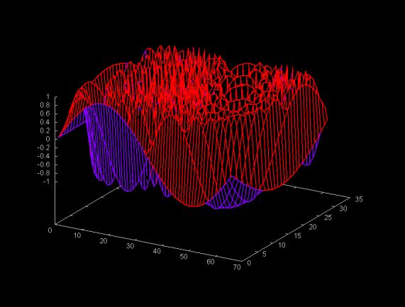
Although this graph is pretty, it is almost entirely un-informative. However, it we look at the data used to generate the graph we can notice that sine values for m=2 on can be derived by striding through the values in the first array, where m=1. Here every other values is taken from the m=1 array and we wrap around to the start of the array when we reach the end. The m=3 sine values can be derived by taking every third value, etc... This is shown in the table below.
| m = 1 | 0.0 | 0.09505 | 0.18925 | 0.28173 | 0.37166 | 0.45822 | 0.54064 | 0.61815 | 0.69007 | 0.75574 | 0.81457 | 0.86602 | 0.90963 |
| m = 2 | 0.0 | 0.18925 | 0.37166 | 0.54064 | 0.69007 | 0.81457 | 0.90963 | ||||||
| m = 3 | 0.0 | 0.28173 | 0.54064 | 0.75574 | 0.90963 | m = 4 | 0.0 | 0.37166 | 0.69007 | 0.90963 |
The constructor for the Java fasterdft class is passed a Vector containing the sample points over with the DFT will be calculated. The constructor initializes two arrays one with cosine value, for n=0..N-1: cos((2Pi*n)/N) and another array containing the sine values for n=0..N-1: sin((2Pi*n)/N). For a DFT point at m, the sine and cosine values can be derived by striding through these arrays. This removes sine and cosine calculation from the loop used to calculate a DFT value. The Java for the DFT loop is shown below.
	for (int n = 0; n < N; n++) {
	  p = (point)data.elementAt( n );
	  x = p.y;
	  int index = (n * m) % N;
	  double c = cosine[ index ];
	  double s = sine[ index ];
	  R = R + x * c;
	  I = I - x * s;
	} // for
The Java code for the fasterdft class can be downloaded here
SIMD stands for Single Instruction, Multiple Data. Back before the killer micros caused the first supercomputer die-off, there were two companies, MasPar and Thinking Machines, which sold massively parallel SIMD processors. This is not the place for a long digression on SIMD parallel processors and algorithms. Briefly SIMD systems consist of large arrays of processors where each processor executes the same instruction or sits out the instruction cycle and does nothing. Whether a processor executes the current instruction depends on the value of a bit which can be set conditionally. The processors are interconnected via a multistage communication network, so at each cycle processors a processor can send values to another processors.
Using an array of N SIMD processors, and N point DFT can be calculated in Olog2N steps. This is considerably faster than the FFT, but performance is bought with hardware. In an age of cheap VLSI this may not be too high a price to pay for some applications.
Ian Kaplan, October 2001
Revised:
Back to A Notebook Compiled While Reading Understanding Digital Signal Processing by Lyons