Click on an image below to view a larger version
Markowitz's mean-variance optimization, first published in 1955, laid the foundation for quantitative equity portfolio construction. Many people fall a bit in love with Markowitz's mean-variance optimized portfolios.
The mathematical derivation of the global minimum variance portfolio, using Lagrange multipliers is elegant.
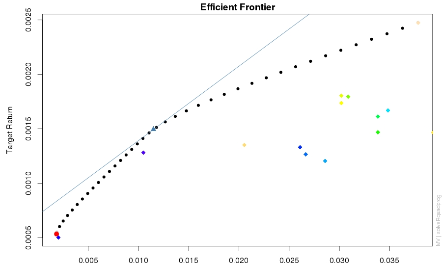
By adjusting the target portfolio return, the efficient frontier for the portfolio can be generated. According to the mean-variance theory, the portfolios that lie along the curve of the efficient frontier have the maximum return for a given variance (on the x-axis).
The tangency portfolio, which is the point on the efficient fronter that is tangent to a line from the risk free rate of return (on the y-axis) is the portfolio with the maximum Sharpe ratio (the portfolio with the highest ratio of return to risk).
In my graduate portfolio construction class one of my classmates was so enamored with mean-variance optimization that he calculated optimized portfolios for his 401K retirement account.
The early romance with Markowitz's mean-variance optimization soon runs into the criticism of mean-variance optimization in the finance literature.
The equation to estimate the portfolio weights is derived from the mean variance equation shown below.
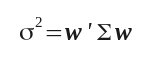
In Markowitz's mean variance optimization, the covariance matrix, sigma, is estimated from a matrix of historical asset returns (for large portfolios there can be problems calculating the covariance matrix and inverting it, which is an issue that I am not going to discuss here). The result of the mean-variance optimization is a set of portfolio weights (which sum to one) for a given mean portfolio return and an estimate of the portfolio variance. These values are calculated over the historical period used to build the covariance matrix. The assumption is that the mean return and variance are stable values (a portfolio with the estimated weights will have the estimated mean return and variance for some time in the future).
For the mean and variance to be stable, the return distributions for the portfolio assets would have to be stable and have a Gaussian distribution. However, this is frequently not true. In many cases the return distributions have "fat tails" and are skewed. The covariance between portfolio assets returns (which can also be represented as correlation) is also not stable in many cases.
This suggests that a matrix of historical returns can be a poor predictor for the future portfolio mean return and variance [1]. One reason that multi-factor models [2] are popular is that the result of the factor model, which can be used to construct the covariance matrix, can be a better predictor of future mean returns.
Although mean-variance portfolio optimization, using historical returns, has been criticized, there is good support in R for constructing mean-variance portfolios. Mean-variance portfolios are the path of least resistance when it comes to portfolio construction.
I wanted to gain a better understanding of how well (or poorly) mean-variance optimization does in estimating portfolio returns. This result provides a baseline against which possibly better methods can be measured.
I also wanted to investigate whether a portfolio with better investment characteristics than a simple index fund could be constructed using mean variance optimization. Again, the mean-variance results serve as a baseline for other methods.
Portfolios constructed by professional portfolio managers are usually constructed from a large universe of individual stocks. Frequently this universe consists of hundreds or even thousands of stocks, which are filtered down using portfolio construction software. This software allows the portfolio manager to select stocks by industry and other factors.
Constructing a portfolio from a relatively large set of stocks avoids high concentrations in a few stocks (usually the portfolio optimization software allows maximum concentration limits to be placed on the portfolio).
In this experiment I used R and historical price data downloaded from Yahoo. Building a large universe of stocks and the necessary filtering infrastructure seemed like a daunting task (although position limits are pretty easy to implement with the tseries function portfolio.optim()).
Instead of using individual stocks, I used Exchange Traded Funds (ETFs). ETFs have the characteristics of index funds or mutual funds, but they are traded like stocks (with trading commissions like those for stocks). ETFs do not have a minimum investment amount as mutual funds frequently do. Like mutual funds, ETFs do have a management fee, which is charged against fund assets.
Most ETFs are constructed from categories or indexes (e.g., consumer commodity stocks or the Russell 1000 Small Cap Stock Index). ETFs are already diversified, so it is not a problem if the portfolio optimizer puts a high concentration of the portfolio in one ETF.
In this experiment I wanted enough history to allow me to draw valid conclusions, so I choose ETFs that has a history of at least ten years. ETFs are relatively new and some of the more interesting ETFs have only been available for a year or two. This limited the ETFs that I could choose from.
The ETF portfolio assets are shown below. The SPY ETF is not included in the portfolio but serves as a proxy for the "market" (in this case the S&P 500).
| ETF Symbol | Description |
|---|---|
| LQD | iShares investment grade corporate bond |
| SHY | iShares Barclays 1-3 Year Treasury Bond |
| IWF | Russell 1000 Large Cap Growth Index Fund |
| IWB | Russell 1000 Large Cap Market Index |
| IWD | Russell 1000 Large Cap Value Index Fund |
| IWO | Russell 2000 Small Cap Growth Index |
| IWM | Russell 2000 Small Cap Index |
| IWN | Russell 2000 Small Cap Value Index |
| IWP | Russelll Midcap Growth Index Fund |
| IWR | Russelll Midcap Index Fund |
| IWS | Russelll Midcap Value Index Fund |
| IYM | Dow Jones US Basic Materials Sector |
| IYK | Dow Jones Consumer Goods |
| IYE | Dow Nones US energy Sector |
| SPY | State Street SPDR S&P 500 (proxy for "the market") |
In this experiment, I calculated weekly log returns from historical weekly close price data, downloaded from finance.yahoo.com (the R script I used is included below).
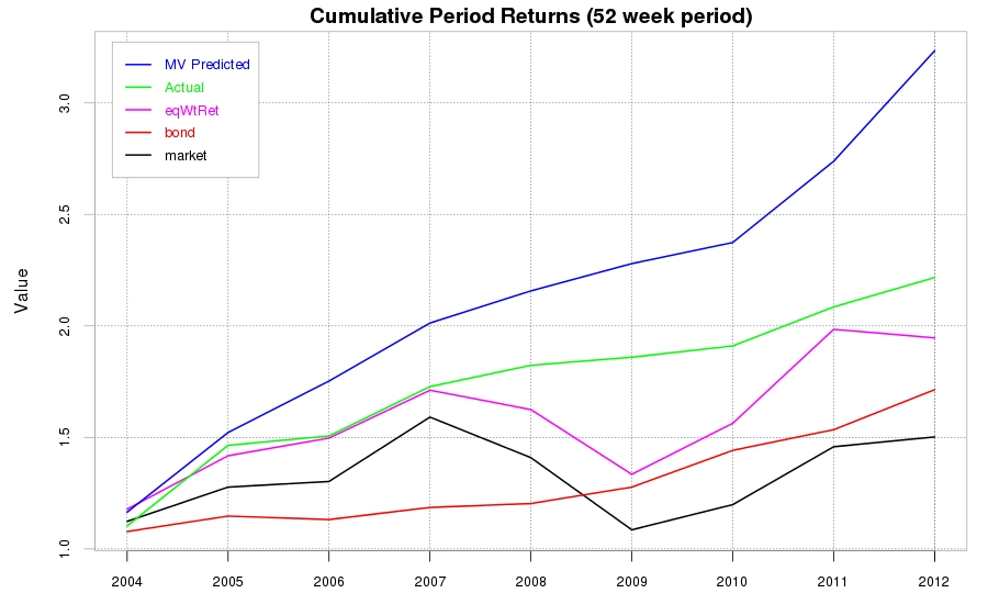
I calculated the portfolio weights, mean return and variance for a long-only, maximum Sharpe ratio portfolio. I then moved N weeks into the future and calculated the actual (out-of-sample) portfolio return. I wrote code to calculate the out-of-sample mean return and period return (e.g., buy at the start of the period and sell at the end of the period). The results were very similar and I have used period return the cumulative return and draw down plots, below.
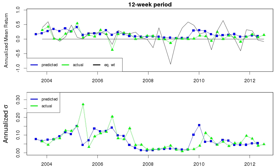
I used weekly returns because they provide more data than monthly returns. However, weekly returns are problematic when it comes to representing the portfolio return. We commonly think of returns on an annual basis, not a weekly basis, so I have annualized the returns. In some cases this seems to give outlandish returns. Weekly returns can be highly variable, which results in highly variable and probably over-estimated, annualized returns.
Two periods were used: one year and one quarter (12 weeks). That is, a portfolio was estimated and then the out-of-sample period (of a year or a quarter) was calculated. Then the year long portfolio windows is moved forward one period and a new portfolio is calculated (e.g., the portfolio is rebalanced).
A year period was used because this is a common choice for portfolios for tax reasons (profits from investments that are held for longer than a year are taxed at a lower rate)
A portfolio that is rebalanced only once a year (or a year and a day) may miss significant changes in the market. By re-balancing more frequently a more optimal portfolio can be obtained. However, there are tax costs. Re-balancing quarterly seems to be a reasonable compromise that catches market changes and keeps portfolio turnover relatively low.
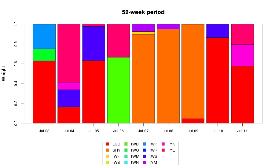
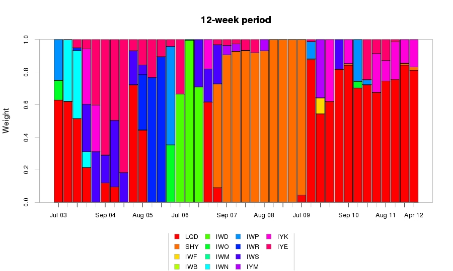
The bar-plot shows how the portfolio weights changed over time.

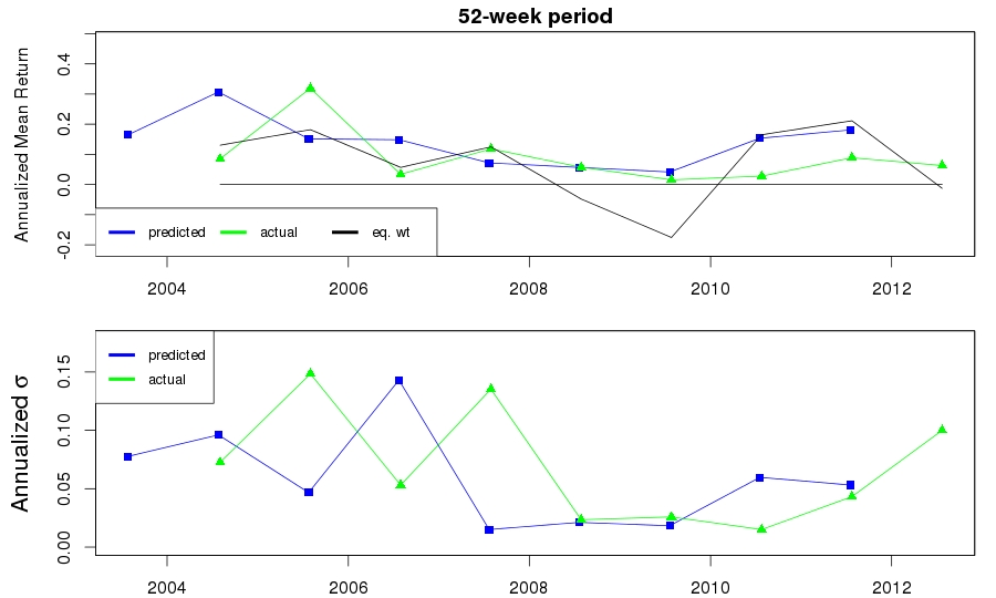
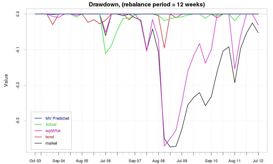
Note that the estimated maximum Sharpe ratio portfolio constructed using mean-variance optimization never loses money, so there is no draw-down (the blue line is flat). Obviously this is not a realistic estimate.
The results show that the mean return and variance estimated by mean-variance optimization is a poor predictor for the actual portfolio mean and variance. Mean-variance optimization over estimates the return and, to a lesser degree, underestimates the variance.
Although mean-variance optimization does not provide accurate estimates for the return and variance, it was used to construct a portfolio that has better performance than comparison portfolios (an equally weighted portfolio, a bond portfolio and the S&P 500). This portfolio doubles the investment in approximately ten years, with limited draw-down and variance.
The portfolio estimation can be improved in a number of ways. This would, hopefully, result in an optimized portfolio that does a better job of estimating return and risk (variance or ETL). Future work includes:
Use mean-ETL optimization, instead of mean variance optimization.
The maximum Sharpe ratio portfolios are optimized for mean/variance. A problem with mean-variance optimization is that it assumes that the tails of the distribution curve are symmetric. In many cases this is not true. If, for example, there is a distribution that is skewed toward positive return, then mean-variance will assume that there is a symmetric negative tail to the distribution. Mean-Expected Tail Loss (ETL) optimizes with respect to the negative tail. Instead of the Sharpe ration, the STARR ratio is used. This is the ratio of excess return to ETL.
The comparison portfolios allow the optimized portfolio to be compared to various benchmarks. After all, if the benchmark performs better than the optimized portfolio then then benchmark will be chosen as an investment asset.
The "equally weighted" portfolio, which is used for comparison in the above plots is weighted heavily toward the equity ETFs. A better comparison might be a 50/50 equity/bond portfolio (or some other fixed percentage, like 60/40).
The portfolios that I have modeled here are long-only portfolios. These portfolios miss possibly profiting from downside price movements, so it would be worth investigating long-short portfolios (short positions can be taken in some ETFs).
The result produced by the analytic Markowitz portfolio equations is a long-short portfolio, where the weights sum to 1, but some weights may be negative.
The assumption in these long-short portfolios is that the proceeds from the short position (where a stock is borrowed and then sold, to be replaced at some time in the future) is used to partially fund the long positions. This is an academic model that only works for investment banks with AA credit ratings. When those of us who are not investment banks short a stock, the proceeds of the short are held in a margin account and cannot be used to purchase a long position.
The reality of shorting makes it more complex than the academic model but it would probably still improve portfolio return, although possibly at the cost of extra variance.
In the last few years a large variety of ETFs have become available. There are ETFs with high beta, ETFs with low beta, ETFs that are constructed using the Axioma optimizer, 130/30 long-short ETFs and sector ETFs. Drawing from a wider universe of ETFs it may be possible to select a portfolio that has higher return.
Mean-variance optimization attempts to predict the future mean and variance of the portfolio. Mean-variance optimization based on historical returns suffers from the problem that historical returns can be a poor predictor for future returns. When the covariance matrix is estimated from historical returns, the result suffers from this drawback as well.
One of the simplest ways to improve the predictive power of the historical returns used to build the covariance matrix is to filter the historical returns using the exponentially weighted moving average (EWMA) function [1][3].
Multi-factor models can also be used for better covariance matrix estimation. Multi-factor models are used for portfolios of stocks. It is not clear that a multi-factor model would apply to a portfolio of ETFs, which are already diversified. However, the components of the ETFs could be decomposed into individual stocks, which could then be used to build a factor-model based portfolio.
Autocorrelation provides one measure for the predictive power of a time series. For portfolios the Information Ratio and Information Coefficient are also good measures for the relationship between the model prediction and the actual values.
I would like to think Professor Doug Martin for his portfolio construction course at the University of Washington and his patient discussion of portfolio construction outside of the course.
I would also like to thank Brian Ertley for his comments and insight into portfolio construction.
Any errors are, of course, mine.
1. Chapter 6, Behavioral Investment Management: An Efficient Alternative to Modern Portfolio Theory by Greg B. Davies and Arnaud de Servigny, McGraw-Hill 2012
2. Chapter 15, Modeling Financial Time Series with S-Plus, Second Edition, Eric Zivot and Jiahui Wang, Springer 2006
3. Professor Doug Martin, University of Washington, Portfolio Optimization and Asset Management, Notes for Lecture 16.R source code: etf_portfolio.r
R code Listing:
# A small set of ETF shares were selected for this experiment. To allow a rolling window # I wanted as long a history as possible. ETFs are relatively new instruments, so there # where a limited number that had an approximately ten year history. # # LQD iShares investment grade corporate bond # SHY iShares Barclays 1-3 Year Treasury Bond # # IWF Russell 1000 Large Cap Growth Index Fund # IWB Russell 1000 Large Cap Market Index # IWD Russell 1000 Large Cap Value Index Fund # # IWO Russell 2000 Small Cap Growth Index # IWM Russell 2000 Small Cap Index # IWN Russell 2000 Small Cap Value Index # # IWP Russelll Midcap Growth Index Fund # IWR Russelll Midcap Index Fund # IWS Russelll Midcap Value Index Fund # # IYM Dow Jones US Basic Materials Sector # IYK Dow Jones Consumer Goods # IYE Dow Jones US energy Sector # # Proxy for the market: # # SPY State Street SPDR S&P 500 # # Author: Ian L. Kaplan # September 2012 # # This code is in the public domain. This code is research code and is not intended to be used # for actual investment. This code is published without warranty and the user accepts all risk # in using this code. # library("PerformanceAnalytics") library("tseries") library("colorspace") # # Build a matrix of market quotes. The fuction returns the quotes as a zoo # matrix. # Arguments: # symbols- a vector of one or more symbols (character strings) # period - d (daily), w (weekly) or m (monthly) # startDate - start date in ISO date format (e.g., 2011-12-31) # endDate - end date in ISO date format # buildQuoteMatrix = function( symbols, period, startDate, endDate) { for (i in 1:length(symbols)) { sym = symbols[i] print(sprintf("Reading symbol %s from yahoo", sym)) ts = get.hist.quote( sym, startDate, endDate, provider="yahoo", compression=period, quote="AdjClose", quiet=T) if (i == 1) { quote.mat = ts } else { quote.mat = cbind(quote.mat, ts) } } colnames(quote.mat) = symbols return( quote.mat) } # buildQuoteMatrix # # Calculate the weekly rate for an annual interest time series # symbol - the symbol for the interest rate instrument (e.g., ^TNX for the ten year t-note) # startDate, endDate - the start and end dates in ISO format # # Note that interest rates are reported as annual rates. Since we're dealing with weekly data, # the annual rate needs to be converted to the weekly rate. # weeklyRate = function( symbol, startDate, endDate) { # get the annual rate, as a percentage rf = get.hist.quote( symbol, startDate, endDate, provider="yahoo", compression="w", quote="AdjClose", quiet=T) rf.frac = rf / 100 rf.week = ((1 + rf.frac)^(1/52)) - 1 return(rf.week) } # # Calculate the long-only tangency portfolio for a returns matrix. The tangency portfolio is # the portfolio with the highest sharp ratio. # longOnlyTangency = function(ret.m, rf) { mu = t(apply(ret.m, 2, mean)) rng = range(mu) minRet = max(rng[1], rf) maxRet = rng[2] nret = 100 retSeq = seq(from=rng[1], to=rng[2], length=nret) sd.vec = c() targetRet = c() weights.l = list() retCov = var(ret.m) ix = 1 minWeight = 0.0 for (i in 1:length(retSeq)) { op = try( portfolio.optim(x=mu, rf=rf, pm=retSeq[i], shorts=F, covmat=retCov), silent=T ) if (class(op) != "try-error") { targetRet = c(targetRet, retSeq[i]) w = op$pw weights.l[[ix]] = round(w,4) sd = sqrt( w %*% retCov %*% w) sd.vec = c(sd.vec, sd) ix = ix + 1 } } weights = matrix(unlist(weights.l), nrow=length(weights.l), ncol=ncol(ret.m), byrow=T) colnames(weights) = colnames(ret.m) sharp = (targetRet - rf) / sd.vec ix = which.max(sharp) tanWeights = weights[ix,] portMu = as.numeric(mu) %*% tanWeights portSd = sd.vec[ix] return(list(w = tanWeights, sd = portSd, mu = portMu)) } # longOnlyTangency # Calculate a long-only, efficient portfolio (using mean variance) and calculate the return # and standard deviation of the forward, out of sample portfolio. # # ret.mat : a matrix of returns # rf.vec : a vector of risk free rates (where length = nrow(ref.mat)) # width : the width of the portfolio window # step : the number of steps to take into the future # # Return # zoo vectors with a date index # predMu : the predicted portfolio return # actMu : the actual portfolio return # predSd : the predicted standard deviation # actSd : the actual standard deviation # eqWt : the mean return of an equally weighted portfolio # # weights : a matrix (with date row names) of portfolio weights # portfolioInOutSample = function( ret.mat, rf.vec, width, step) { numRows = nrow(ret.mat) start = 1 end = width ix = 1 predMu = list() predSd = list() actMu = list() actSd = list() eqWeight = list() weights = list() n = ncol(ret.mat) eqW = rep(1/n, n) while((end + step) < numRows) { window = ret.mat[start:end,] rf = mean(rf.vec[start:end]) t = longOnlyTangency(window, rf) len = nrow(window) y = as.Date(names(window[,1]))[len] predMu[[ix]] = t$mu predSd[[ix]] = t$sd names( predMu[[ix]] ) = y names( predSd[[ix]]) = y w = t$w weights[[ix]] = w outStart = end + 1 outEnd = outStart + step outOfSample = ret.mat[outStart:outEnd,] actRet = as.numeric(outOfSample %*% w) actMu[[ix]] = mean( actRet ) actSd[[ix]] = sd( actRet ) eqWeight[[ix]] = mean(as.numeric(outOfSample %*% eqW)) len = nrow(outOfSample) y = as.Date(names(outOfSample[,1]))[len] names( actMu[[ix]] ) = y names( actSd[[ix]]) = y names( eqWeight[[ix]]) = y start = start + step end = end + step ix = ix + 1 } predMu = unlist(predMu) predSd = unlist(predSd) actMu = unlist(actMu) actSd = unlist(actSd) eqWeight = unlist(eqWeight) predMu.z = as.zoo(predMu) index(predMu.z) = as.Date(names(predMu)) predSd.z = as.zoo(predSd) index(predSd.z) = as.Date(names(predSd)) actMu.z = as.zoo(actMu) index(actMu.z) = as.Date(names(actMu)) actSd.z = as.zoo(actSd) index(actSd.z) = as.Date(names(actSd)) eqWeight.z = as.zoo(eqWeight) index(eqWeight.z) = as.Date(names(eqWeight)) numRows = length(weights) numCols = ncol(ret.mat) weights =matrix(data = unlist(weights), ncol=numCols, nrow=numRows, byrow=T) colnames(weights) = colnames(ret.mat) rownames(weights) = names(predMu) return(list(predMu = predMu.z, actMu = actMu.z, predSd = predSd.z, actSd = actSd.z, eqWt = eqWeight.z, weights = weights)) } # portfolioInOutSample # # - Plot the mean for the predicted, actual and equally weighted portfolio returns, over time # - Plot the predicted and actual standard deviations # - Plot a bar chart showning the portfolio weights over time # # This function takes a list containing the following zoo objects: # predMu : the predicted mean return for the portfolio # actMu : the actual mean return for the portfolio # predSd : the predicted standard deviation for the portfolio # actSd : the actual standard deviation # eqWt : the mean return for the equally weighted portfolio # # weights : this is not a zoo object, but a matrix of portfolio weights over time # plotPortfolios = function( portData, title ) { predMu.z = portData$predMu actMu.z = portData$actMu predSd.z = portData$predSd actSd.z = portData$actSd eqWeight.z = portData$eqWt weights = portData$weights zero = as.zoo(rep(0, length(actMu.z))) index(zero) = index(actMu.z) # Annualize the mean and standard deviation predMu.z = ((1 + predMu.z) ^ 52) - 1 actMu.z = ((1 + actMu.z) ^ 52) -1 eqWeight.z = ((1 + eqWeight.z) ^ 52) - 1 predSd.z = predSd.z * sqrt(52) actSd.z = actSd.z * sqrt(52) minDate = index(predMu.z[1]) maxDate = index(actMu.z[length(actMu.z)]) par(mfrow=c(2,1), mar=c(2,4.5,1.5,1)) ymin = min(predMu.z, actMu.z, eqWeight.z) ymin = ymin - abs(ymin * 0.2) ymax = max(predMu.z, actMu.z, eqWeight.z) ymax = ymax + (ymax * 0.5) plot(predMu.z, type="l", col="blue", main=title, ylab="Annualized Mean Return", ylim=c(ymin, ymax), xlim=c(minDate, maxDate)) lines(zero, type="l", col="black") points(predMu.z, pch=15, col="blue") lines(actMu.z, type="l", col="green") points(actMu.z, pch=17, col="green") lines(eqWeight.z, type="l", col="black") legend(x="bottomleft", legend=c("predicted", "actual", "eq. wt"), col=c("blue", "green", "black"), lwd=4, cex=0.8, horiz=T) minDate = index(predSd.z[1]) maxDate = index(actSd.z[length(actMu.z)]) ymax = max(predSd.z, actSd.z) ymax = ymax + (ymax * 0.2) plot(predSd.z, type="l", col="blue", cex.lab=1.3, ylab=expression(paste("Annualized ", sigma)), xlim=c(minDate, maxDate), ylim=c(0, ymax)) points(predSd.z, pch=15, col="blue") lines(actSd.z, type="l", col="green") points(actSd.z, pch=17, col="green") legend(x="topleft", legend=c("predicted", "actual"), col=c("blue", "green"), lwd=4, cex=0.8, horiz=F) par(mfrow=c(1,1)) par(mfrow=c(1,1)) chart.StackedBar(w = weights, # colorset = rainbow(ncol(weights))[c(seq(from=1, to=ncol(weights), by=2), # seq(from=2, to=ncol(weights), by=2))], colorset = rainbow(ncol(weights)), ylab="Weight", space=0.1, main=title) par(mfrow=c(1,1)) } # plotPortfolios # # Generate cumulative return plots for the portfolio predicted return, the actual return, # the return on a bond ETF and the market return. The portfolio returns are returns over # the number of weeks defined in the weeks argument. The bond and market returns are # weekly returns, which must be aggregated to match the portfolio return # plotPortReturn = function(predMu, actMu, bondMu, mktRet, offset, weeks ) { pMu = coredata(predMu) aMu = coredata(actMu) if (class(mktRet) == "zoo") { mktRet = coredata(mktRet) } # For the bond fund and the market, calculate the mean return over teh weeks window bMu = round(rollapply(bondMu[(offset+1):length(bondMu)], width=weeks, by=weeks, FUN=mean, align="right"), 6) mMu = round(rollapply(mktRet[(offset+1):length(mktRet)], width=weeks, by=weeks, FUN=mean, align="right"), 6) # The returns are the mean return over the weeks period. However, for cumulative returns to work we # need to calculate the compound return over that period. adjPredMu = ((1 + pMu)^weeks) - 1 adjActMu = ((1 + aMu)^weeks) - 1 adjBndMu = ((1 + bMu)^weeks) - 1 adjMktMu = ((1 + mMu)^weeks) - 1 r = cbind(adjPredMu, adjActMu, adjBndMu, adjMktMu) colnames(r) = c("Predicted", "Actual", "Bonds", "S&P 500") par(mfrow=c(1,1)) chart.CumReturns(r, wealth.index=T, main=paste("Cumulative Mean Returns (", weeks, " week period)", sep=""), col=c("blue", "green", "red", "black"), legend.loc="topleft", grid.color="slategrey") par(mfrow=c(1,1)) } # plotPortReturn # # This function attempts to simulate the investment of the MV portfolio by buying at the # start of a period and selling at the end. # # The portfolio is a long-only tangency portfolio. The investment of this portfolio is # simulated by calculating the out-of-sample return over a perios of weeks. The sample used # to calculate is a sliding window of width weeks. # # returns : a matrix of log returns # prices : a matrix of weekly prices # rf : a vector of the weekly risk free rate # width : the width of the window used to estimate the portfolio # weeks : the investment period # W : the initial "wealth" # # The returns used here are defined as # # R = (P[t] - P[t-1])/P[t-1] # # The portfolio is calculated using weekly log returns, so the mean return from the # portfolio calculation is the weekly mean return. # # The out-of-sample return is calculated as if the portfolio were invested at the start # of the period and sold at the end of the period. # # To allow comparison of the out-of-sample return to the portfolio return, the portfolio return # is converted to the return over the period of "weeks". # investmentSimulation = function( returns, prices, rf.vec, width, weeks ) { numRows = nrow(returns) start = 1 end = width ix = 1 predMu = list() portRet = list() eqWtRet = list() n = ncol(returns) eqW = rep(1/n, n) while((end + weeks) < numRows) { window = returns[start:end,] rf = mean(rf.vec[start:end]) t = longOnlyTangency(window, rf) len = nrow(window) y = as.character(rownames(window)[len]) weeklyMu = t$mu periodMu = ((1 + weeklyMu)^weeks) - 1 predMu[[ix]] = periodMu names( predMu[[ix]] ) = y w = t$w outStart = end + 1 outEnd = outStart + weeks # we assume that we buy at the start of the out of sample period (which is just # after the window used to calculate the portfolio) and sell at the end of the # out of sample period R = (prices[outEnd,] - prices[outStart,])/prices[outStart,] portRet[[ix]] = sum( R * w) eqWtRet[[ix]] = sum(R * eqW) y = rownames(prices)[outEnd] names( portRet[[ix]] ) = y names( eqWtRet[[ix]]) = y start = start + weeks end = end + weeks ix = ix + 1 } predMu = unlist(predMu) portRet = unlist(portRet) eqWtRet = unlist(eqWtRet) predMu.z = as.zoo(predMu) index(predMu.z) = as.Date(names(predMu)) portRet.z = as.zoo(portRet) index(portRet.z) = as.Date(names(portRet)) eqWtRet.z = as.zoo(eqWtRet) index(eqWtRet.z) = as.Date(names(eqWtRet)) return(list(predMu = predMu.z, portRet = portRet.z, eqWtRet = eqWtRet.z)) } # investmentSimulation # The returns used here are defined as # # R = (P[t] - P[t-1])/P[t-1] # regionReturn = function( region ) { len = length(region) R = (region[len] - region[1])/region[1] return( R ) } # regionReturn # # Plot the simulated investment portfolios, along with the bond and market returns. # Here the return is the return that would be obtained by buying at the start of # a period and selling at the end of the period. # plotInvest = function( predMu, actRet, eqWtRet, bond, market, window, weeks) { bondRet = rollapply(bond[(window+1):length(bond)], width=weeks, by=weeks, FUN=regionReturn, align="right") mktRet = rollapply(market[(window+1):length(market)], width=weeks, by=weeks, FUN=regionReturn, align="right") retData = cbind(coredata(predMu), coredata(actRet), coredata(eqWtRet), coredata(bondRet), coredata(mktRet)) rownames(retData) = as.character(index(actRet)) colnames(retData) = c("MV Predicted", "Actual", "eqWtRet", "bond", "market") par(mfrow=c(1,1)) chart.CumReturns(retData, wealth.index=T, main=paste("Cumulative Period Returns (", weeks, " week period)", sep=""), col=c("blue", "green", "magenta", "red", "black"), legend.loc="topleft", grid.color="slategrey") par(mfrow=c(1,1)) } plotDrawdown = function( predMu, actRet, eqWtRet, bond, market, window, weeks) { bondRet = rollapply(bond[(window+1):length(bond)], width=weeks, by=weeks, FUN=regionReturn, align="right") mktRet = rollapply(market[(window+1):length(market)], width=weeks, by=weeks, FUN=regionReturn, align="right") retData = cbind(coredata(predMu), coredata(actRet), coredata(eqWtRet), coredata(bondRet), coredata(mktRet)) rownames(retData) = as.character(index(actRet)) colnames(retData) = c("MV Predicted", "Actual", "eqWtRet", "bond", "market") par(mfrow=c(1,1)) chart.Drawdown(retData, main=paste("Drawdown, (rebalance period = ", weeks, " weeks)", sep=""), cex.main=0.8, colorset=c("blue", "green", "magenta", "red", "black"), legend.loc="bottomleft" ) par(mfrow=c(1,1)) } startDate = "2002-08-01" endDate = "2012-08-01" # The universe of Exchange Traded Funds (ETFs) symbols = c("LQD", "SHY","IWF","IWB", "IWD","IWO","IWM","IWN", "IWP", "IWR","IWS", "IYM","IYK", "IYE") # The ten year T-note annual rate rfSym = "^TNX" # Market ETF mktSym = "SPY" returnFile = "etfPrices.R" # Load the ETF returns object, if the save file exists or write out the save file if (file.exists( returnFile ) == T) { load( returnFile ) } else { prices.mat = buildQuoteMatrix(symbols, period="w", startDate, endDate) rfTenYear = weeklyRate(rfSym, startDate, endDate) mkt = get.hist.quote( mktSym, startDate, endDate, provider="yahoo", compression="w", quote="AdjClose", quiet=T) save(prices.mat, mkt, rfTenYear, file=returnFile) } logPrices.mat = apply(prices.mat, 2, log) ret.mat = apply(logPrices.mat, 2, diff) mktRet = diff(log(mkt)) yearPort = portfolioInOutSample(ret.mat, rfTenYear, 52, 52) plotPortfolios( yearPort, "52-week period" ) quarterPort = portfolioInOutSample(ret.mat, rfTenYear, 52, 12) plotPortfolios( quarterPort, "12-week period" ) # Get the weekly bond fund returns, for comparision lqd = ret.mat[,"LQD"] # plotPortReturn(yearPort$predMu, yearPort$actMu, lqd, mktRet, 52, 52) # plotPortReturn(quarterPort$predMu, quarterPort$actMu, lqd, mktRet, 52, 12) prices = coredata(prices.mat) rownames(prices) = as.character(index(prices.mat)) yearInvest = investmentSimulation( ret.mat, prices, rfTenYear, 52, 52) quarterInvest = investmentSimulation( ret.mat, prices, rfTenYear, 52, 12) # weekly prices for the bond fund LQD lqdPrices = prices.mat[,"LQD"] plotInvest(yearInvest$predMu, yearInvest$portRet, yearInvest$eqWtRet, lqdPrices, mkt, 52, 52) plotInvest( quarterInvest$predMu, quarterInvest$portRet, quarterInvest$eqWtRet, lqdPrices, mkt, 52, 12) # # Generate the drawdown plot for the quarterly rebalanced portfolio # plotDrawdown( quarterInvest$predMu, quarterInvest$portRet, quarterInvest$eqWtRet, lqdPrices, mkt, 52, 12) # # Generate the efficient portfolio graph (quick and dirty, since it uses the fPortfolioPackage) # # This function is needed to get around a bug in the fPortfolio portfolioFrontier function # cov = function( mat ) { return(var(mat)) } Constraints = "LongOnly" Spec = portfolioSpec() setNFrontierPoints(Spec) = 80 setRiskFreeRate(Spec) = mean( rfTenYear) ret.mat.ts = as.timeSeries(ret.mat) frontier = portfolioFrontier(data=ret.mat.ts, spec=Spec, constraints=Constraints, description="Long-Only Efficient Frontier") par(mfrow=c(1,1), mar=c(2,4.5,1.5,1)) plot(frontier) par(mfrow=c(1,1)) |
Ian Kaplan
September, 2012
Last updated:
back to Topics in Quantitative Finance
