
In classical Markowitz mean-variance portfolio optimization, efficient portfolios are optimized to minimize variance. Each portfolio along the efficient frontier has the minimum variance for that level of return.
In the distribution of portfolio returns, variance is a double edged blade: there is a down side (e.g., portfolio loss) and an upside (portfolio gain) to the variance distribution. Minimizing the variance penalizes for both the downside and the upside of the distribution.
A CVaR optimized portfolio only penalizes for the loss, not the gain in the portfolio return distribution.
CVaR stands for Conditional Value at Risk. For some reason, CVaR has the aliases: ETL - Expected Tail Loss and ES - Expected Shortfall.
CVaR is a down side risk measure. It is related to Value at Risk, VaR, but is a better risk measure for several reasons. Value at Risk describes a loss of X or greater. This last clause tends to be omitted when people quote VaR. CVaR is an estimate of the size of the tail loss, which gives a more accurate estimate of the risk.
As is the case with calculating VaR, calculating CVaR has its challenges. Calculating the 5% CVaR (e.g., the 1 in 20 chance of a loss) involves estimating the tail of the distribution. If a Gaussian distribution is assumed then this can be done analytically. However, this can be problematic since many financial time series have fat tails and a Gaussian distribution seriously underestimates the size of the tail. CVaR can also be estimated from historical data. An R algorithnm for historical CVaR estimation is shown below. However, in most cases there are relatively few points that make up the 5% tail distribution, so this estimate is imperfect as well.
# # Calculation of ETL/ES/CVaR # library("fEcofin") library("zoo") library("PerformanceAnalytics") data("sp500index") tradingDays = 252 years = 3 days = tradingDays * years end = dim(sp500index)[1] start = end - (days-1) sp500 = sp500index[start:end,] d = sp500[,1] dates = as.Date(d) close = sp500[,2] close.z = zoo(close, dates) sp500.ret.z = diff(log(close.z)) # # Calculate historical CVaR # CVaR <- function (r, alpha = 0.05) { x = as.matrix(r) etl = mean(sort(x)[1:round(length(x) * alpha)]) return(etl) } cvar = CVaR(sp500.ret.z) etl = ETL(sp500.ret.z, method="historical") print(sprintf("CVaR (historical) = %1.5f, etl (historical) = %1.5f", cvar, etl)) |
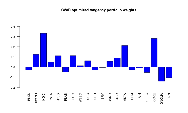
The weights for the long/short minimum-CVaR tangency portfolio are shown below.
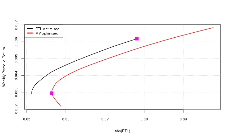
The plot below shows two portfolio frontiers: a frontier minimizing CVaR and a frontier minimizing variance (e.g., the classic Markowitz mean-variance frontier). In the case of the mean-variance frontier, the 5% CVaR value was calculated for each of the portfolios that are plotted on the frontier. The points on the plot show the CVaR tangency portfolio and the global minimum variance portfolio.
The mean-variance optimized portfolios are overly constrained since they are penalized for the portfolio upside as well as the downside. The CVaR optimized portfolios are only penalized for the downside risk and dominate the mean-variance portfolios (e.g., for every level of down side risk there is a CVaR optimized portfolio with a higher return than the mean-variance portfolio).
The R code that calculated the efficient frontiers is included below. For an unconstrained long/short portfolio, there is an analytic solution for the mean-variance optimization problem. There is no analytic solution for a CVaR minimized portfolio. The solution can only be calculated numerically, using numeric optimization.
The R script below uses the fPortfolio library from rmetrics. I used the fPortfolio library because it suports CVaR minimized portfolios.
I am grateful that Rmetrics has made their software libraries freely available to the R community. However, I found the fPortfolio library buggy and difficult to use. For example, I could not get the limit constraint to work for long-only portfolios.
The fPortfolio documentation is limited and it can be difficult to understand how to use the functions in the library. There is an eBook published by Rmetrics, but it is quite expensive (about $120 US at the time this was written). From looking at parts of this book on Google books I'm not sure that the book would be worth the cost to me. While I think that the Rmetrics work should be supported, I can't afford to support them at this level.
The fPortfolio functions seem to be targeted at long-only portfolios. Although I was able to use the functions to calculate long/short CVaR minimized portfolios, I was unable to use the functions to calculate long/short mean-variance portfolios. I used the analytic solution for these portfolios to calculate the efficient mean-variance frontier.
R code: etl_opt.r
Data: smallcap_weekly.csv
# # Basic ETL optimization, using fPortfolio and an analytic global minimum variance # portfolio for comparision. The analytic GMV was used because fPortfolio seems to be # broken when it comes to calculating a GMV portfolio with shorts allowed. # # Author: Ian Kaplan # rm(list=ls()) library("zoo") library("fPortfolio") library("PerformanceAnalytics") # # This function is passed a matrix of returns. The result is # the weights, mean return and standard deviation of the # global minimum variance portfolio, where the only # constraint is full investment (e.g., shorting is allowed). # analyticGMV = function(returns) { S = cov(returns) Sinv = solve(S) one = rep(1, ncol(S)) denom = as.numeric(t(one) %*% Sinv %*% one) w = (Sinv %*% one) / denom sd = 1 / sqrt(denom) rslt = list(w = round(t(w), 8), mu = mean(returns %*% w), sd = sd) return(rslt) } # # Calculate the weights, mean return and standard deviation of the # tangency portfolio. # analyticTangency = function(returns, rf) { mu = apply(returns, 2, mean) S = cov(returns) Sinv = solve(S) one = rep(1, ncol(S)) mu_e = mu - rf w = (Sinv %*% mu_e) / as.numeric((t(one) %*% Sinv %*% mu_e)) sd = sqrt(t(w) %*% S %*% w) rslt = list(w = round(t(w), 6), mu = sum(w * mu), sd = sd) return(rslt) } # # Given two Markowitz mean/variance optimized portfolio weights, calculate a set of # means and 5% CVaR values for the efficient frontier using the "two fund theorm". # Note that these are not CVaR optimized portfolio. The CVaR value is calculated # from the weighted return distribution. # meanETLPoints = function(returns, gmv_wts, tan_wts, alpha = seq(from=-0.1, to=1.1, by=0.05)) { y_mu = list() x_etl = list() gmv_wts_t = as.vector(gmv_wts) tan_wts_t = as.vector(tan_wts) C = cov(returns) ix = 1 mu = apply(returns, 2, mean) for (i in alpha) { w = i * gmv_wts_t + ((1-i) * tan_wts_t) y_mu[ix] = mu %*% w x_etl[ix] = cvarRisk(returns, w) ix = ix + 1 } rslt = list(mu=y_mu, etl=x_etl) return(rslt) } # # Calculate the efficient frontier for CVaR (ETL) optimized portfolios between a mininum mean # and a maximum mean. This is done by calculating portfolios for a given target return. # etlPoints = function(returns.ts, minMu, maxMu ) { spec = portfolioSpec() setType(spec) = "CVaR" constraints = "Short" nPts = 40 muRange = seq(from=minMu, to=maxMu, by=((maxMu - minMu)/nPts)) mu = list() etl = list() for (i in 1:length(muRange)) { targetMu = muRange[i] setTargetReturn( spec ) = targetMu port = efficientPortfolio(data=returns.ts, spec=spec, constraints=constraints) mu[i] = targetMu etl[i] = cvarRisk(returns.ts, getWeights(port)) } rslt = list(mu = mu, etl = etl) } # # Read in a small cap. stock return data set and convert the dates into the ISO format used for a # zoo date index. The last two columns a "market" data set and the weekly risk free rate # (T-bill rate) # smallCap.z = read.zoo(file="smallcap_weekly.csv", sep=",", header=T, format = "%m/%d/%Y") smallCapWin.z = window(smallCap.z, start="2000-01-01") market = smallCapWin.z[,"Weekvwretd"] rf = smallCapWin.z[,"WeekRiskFree"] stocks.z = smallCapWin.z[,1:(ncol(smallCap.z)-2)] stocks.ts = as.timeSeries(stocks.z) mu = apply(stocks.ts, 2, mean) spec = portfolioSpec() setType(spec) = "CVaR" setRiskFreeRate(spec) = mean(rf) constraints = "Short" # Calculate the CVaR (ETL) optimized tangency portfolio weights tan.etl = tangencyPortfolio(data=stocks.ts, spec = spec, constraints = constraints) # calculate the CVaR (ETL) optimized global minimum variance portfolio weights gmv.etl = minvariancePortfolio(data=stocks.ts, spec=spec, constraints=constraints) # wts.tan.etl = getWeights(tan.etl) names(wts.tan.etl) = colnames(stocks.ts) # wts.gmv.etl= getWeights(gmv.etl) names(wts.gmv.etl) = colnames(stocks.ts) # gmv.etl.mu = mu %*% wts.gmv.etl tan.etl.mu = mu %*% wts.tan.etl # # Calculate the analytic Markowitz tangency portfolio weights wts.tan.mv = analyticTangency( stocks.ts, mean(rf) )$w # Calculate the Markowitz global minimum variance portfolio weights t = analyticGMV( stocks.ts ) wts.gmv.mv = t$w # Calculate the efficient Markowitz frontier, except with abs(ETL) on the x-axis mvPlot = meanETLPoints(stocks.ts, wts.gmv.mv, wts.tan.mv ) mv.mu = as.numeric(mvPlot$mu) mv.etl = abs(as.numeric(mvPlot$etl)) gmv.mu = mv.mu[ which.min(mv.etl)] gmv.etl = mv.etl[ which.min(mv.etl)] # Calculate the efficient CVaR optimized frontier etlPlot = etlPoints(stocks.ts, gmv.etl.mu, tan.etl.mu ) etl.mu = as.numeric(etlPlot$mu) etl.etl = abs(as.numeric(etlPlot$etl)) tan.mu = tan.etl.mu tan.etl = cvarRisk(stocks.ts, wts.tan.etl) par(mfrow=c(1,1)) xmin = min(etl.etl, mv.etl) xmax = max(etl.etl, mv.etl) ymin = min(etl.mu, mv.mu) ymax = max(etl.mu, mv.mu) plot(x=etl.etl, y=etl.mu, xlim=c(xmin, xmax), ylim=c(ymin, ymax), type="l", col="black", ylab="Weekly Portfolio Return", xlab="abs(ETL)", lwd=2 ) lines(x = mv.etl, y=mv.mu, type="l", col="red", lwd=2) points(x = c(abs(gmv.etl), abs(tan.etl)), y = c(gmv.mu, tan.mu), col="magenta", cex=1.5, pch=15) grid(col="grey") legend(x="topleft", legend=c("ETL optimized", "MV optimized"), col=c("black", "red"), lwd=4) par(mfrow=c(1,1)) |
Ian Kaplan
June, 2012
Last updated:
back to Topics in Quantitative Finance