@(#)QSortAlgorithm.java 1.3 29 Feb 1996 James Gosling
Copyright (c) 1994-1996 Sun Microsystems, Inc. All Rights Reserved.
Permission to use, copy, modify, and distribute this software and its documentation for NON-COMMERCIAL or COMMERCIAL purposes and without fee is hereby granted.
Please refer to the file http://www.javasoft.com/copy_trademarks.html for further important copyright and trademark information and to http://www.javasoft.com/licensing.html for further important licensing information for the Java (tm) Technology.
*/ public class qsort { /** This is a generic version of C.A.R Hoare's Quick Sort * algorithm. This will handle arrays that are already * sorted, and arrays with duplicate keys.* * If you think of a one dimensional array as going from * the lowest index on the left to the highest index on the right * then the parameters to this function are lowest index or * left and highest index or right. The first time you call * this function it will be with the parameters 0, a.length - 1. * * @param a an integer array * @param lo0 left boundary of array partition * @param hi0 right boundary of array partition */ static void QuickSort(double a[], int lo0, int hi0) { int lo = lo0; int hi = hi0; double mid; if ( hi0 > lo0) { /* Arbitrarily establishing partition element as the midpoint of * the array. */ mid = a[ ( lo0 + hi0 ) / 2 ]; // loop through the array until indices cross while( lo <= hi ) { /* find the first element that is greater than or equal to * the partition element starting from the left Index. */ while( ( lo < hi0 ) && ( a[lo] < mid ) ) ++lo; /* find an element that is smaller than or equal to * the partition element starting from the right Index. */ while( ( hi > lo0 ) && ( a[hi] > mid ) ) --hi; // if the indexes have not crossed, swap if( lo <= hi ) { swap(a, lo, hi); ++lo; --hi; } } // while /* If the right index has not reached the left side of array * must now sort the left partition. */ if( lo0 < hi ) QuickSort( a, lo0, hi ); /* If the left index has not reached the right side of array * must now sort the right partition. */ if( lo < hi0 ) QuickSort( a, lo, hi0 ); } } // QuickSort private static void swap(double a[], int i, int j) { double T; T = a[i]; a[i] = a[j]; a[j] = T; } // swap public static void sort(double a[]) { QuickSort(a, 0, a.length - 1); } // sort } // qsort �������������wavelets/sortTest.java������������������������������������������������������������������������������100644 � 1040 � 1001 � 6207 7321423165 13605� 0����������������������������������������������������������������������������������������������������ustar ���������������������������������everyone��������������������������������������������������������������������������������������������������������������������������������������������������������������������������������������������������������������� import java.util.Random; import sort.*; /**
Test for generic sort
Classes to sort a specific type are derived from the abstract generic_sort class. This code tests the sort code by creating two specific sort classes: one that sorts arrays of testElem objects by index and one that sorts by the val field.
*/ class sortTest { /**Test data structure: index is the array index and val is the data element.
An array of testElem objects can be sorted by value and than rearranged back into the original order by sorting by index.
*/ private class testElem { testElem( int i ) { index = i; } public int index; public double val; } /** Sort by index */ private class sort_testElem_index extends generic_sort { /** if (a.index == b.index) return 0 if (a.index < b.index) return -1 if (a.index > b.index) return 1; */ protected int compare( Object a, Object b ) { int rslt = 0; testElem t_a = (testElem)a; testElem t_b = (testElem)b; if (t_a.index < t_b.index) rslt = -1; else if (t_a.index > t_b.index) rslt = 1; return rslt; } // compare } // sort_testElem_index /** Sort by value */ private class sort_testElem_val extends generic_sort { /** if (a.val == b.val) return 0 if (a.val < b.val) return -1 if (a.val > b.val) return 1; */ protected int compare( Object a, Object b ) { int rslt = 0; testElem t_a = (testElem)a; testElem t_b = (testElem)b; if (t_a.val < t_b.val) rslt = -1; else if (t_a.val > t_b.val) rslt = 1; return rslt; } // compare } // sort_testElem_val public sort_testElem_val alloc_sort_testElem_val() { return new sort_testElem_val(); } public sort_testElem_index alloc_sort_testElem_index() { return new sort_testElem_index(); } public testElem[] alloc_array( int size ) { testElem a[] = new testElem[ size ]; for (int i = 0; i < size; i++) { a[i] = new testElem( i ); } return a; } void printArray( testElem a[] ) { for (int i = 0; i < a.length; i++) { System.out.println(i + " " + a[i].index + " " + a[i].val ); } } public static void main( String[] args ) { sortTest s = new sortTest(); final int size = 20; testElem a[] = s.alloc_array( size ); Random generator = new Random(); for (int i = 0; i < a.length; i++) { a[i].val = generator.nextDouble(); } sort_testElem_index sortByIndex = s.alloc_sort_testElem_index(); sort_testElem_val sortByVal = s.alloc_sort_testElem_val(); System.out.println("before sort by val"); s.printArray( a ); sortByVal.sort( a ); System.out.println("after sort by val"); s.printArray( a ); sortByIndex.sort( a ); System.out.println("after sort by index"); s.printArray( a ); } } // sortTest �����������������������������������������������������������������������������������������������������������������������������������������������������������������������������������������������������������������������������������������������������������������������������������������������������������������������������������������������������������������������������������������wavelets/spectrum_test.java�������������������������������������������������������������������������100644 � 1040 � 1001 � 2056 7321424367 14662� 0����������������������������������������������������������������������������������������������������ustar ���������������������������������everyone��������������������������������������������������������������������������������������������������������������������������������������������������������������������������������������������������������������� import java.io.*; import wavelets.*; import wavelet_util.*; import dataInput.*; /** Generate gnuplot files for the time series with various spectrum removed. */ class spectrum_test { public static void main( String[] args ) { String timeSeriesFile = "amat_close"; // Applied Materials Close prices tsRead data = new tsRead( timeSeriesFile ); // // The wavelet algorithms work on arrays whose length is a power // of two. Set the length to the nearest power of two that is // less than or equal to the data length. // int len = data.getSize(); if (len > 0) { int newSize = binary.nearestPower2( len ); data.setSize( newSize ); double[] vals = data.getArray(); if (vals != null) { wavelets.inplace_haar haar = new wavelets.inplace_haar(); haar.wavelet_calc( vals ); haar.order(); coef_spectrum spectrum = new coef_spectrum(); spectrum.filter_one_spectrum( vals ); spectrum.only_one_spectrum( vals ); } } } } // spectrum_test ����������������������������������������������������������������������������������������������������������������������������������������������������������������������������������������������������������������������������������������������������������������������������������������������������������������������������������������������������������������������������������������������������������������������������������������������������������������������������������wavelets/statTest.java������������������������������������������������������������������������������100644 � 1040 � 1001 � 3114 7321423552 13563� 0����������������������������������������������������������������������������������������������������ustar ���������������������������������everyone��������������������������������������������������������������������������������������������������������������������������������������������������������������������������������������������������������������� import dataInput.*; import wavelets.*; import wavelet_util.binary; import experimental.*; /** Test the experimental code to generate a normal curve with the mean and standard deviation derived from a coefficient spectrum (in this case the highest frequency spectrum). */ class statTest { public static void print_curve( statistics.bell_info info, statistics.point curve[] ) { System.out.println("#"); System.out.println("# mean = " + info.mean ); System.out.println("# stddev = " + info.sigma ); System.out.println("#"); for (int i = 0; i < curve.length; i++) { System.out.println( curve[i].x + " " + curve[i].y ); } System.out.println(); } public static void main( String[] args ) { tsRead ts = new tsRead("amat_close"); int len = ts.getSize(); if (len > 0) { len = binary.nearestPower2(len); ts.setSize( len ); double vals[] = ts.getArray(); wavelets.inplace_haar haar = new inplace_haar(); haar.wavelet_calc( vals ); haar.order(); int end = vals.length; int start = end >> 1; double coef[] = new double[ start ]; int ix = 0; for (int i = start; i < end; i++) { coef[ix] = vals[i]; ix++; } statistics.bell_info info = statistics.stddev( coef ); if (info != null) { statistics.point curve[] = statistics.normal_curve(info, start); // print_curve( info, curve ); statistics stat = new statistics(); stat.integrate_curve( curve ); } } } // main } // statTest ����������������������������������������������������������������������������������������������������������������������������������������������������������������������������������������������������������������������������������������������������������������������������������������������������������������������������������������������������������������������������������������������������������������������������������������������������wavelets/timeseries_histo.java����������������������������������������������������������������������100644 � 1040 � 1001 � 6107 7314667101 15336� 0����������������������������������������������������������������������������������������������������ustar ���������������������������������everyone��������������������������������������������������������������������������������������������������������������������������������������������������������������������������������������������������������������� import wavelets.*; import wavelet_util.*; import experimental.*; import dataInput.*; /**Generate histograms for the Haar coefficients created by applying the Haar transform to the time series for the Applied Materials (symbol: AMAT) daily close price.
There are 512 data points in the AMAT daily close price time series. This program generates a histogram for the first four high frequency sets of coefficients (e.g., 256, 128, 64, and 32 coefficients).
Financial theory states that the average daily return (e.g, the difference between today'ss close prices and yesterday's close price) is normally distributed. So the histogram of the highest frequency coefficients, which reflect the difference between two close prices, should be bell curve shaped, centered around zero.
The close price in the AMAT time series rises sharply about half way through. So as the coefficient frequency decreases, the histogram will be shifted farther and farter away from zero.
Note that an inplace Haar transform is used that replaces the values with the coefficients. The order function orders the coefficients from the butterfly pattern generated by the inplace algorithm into increasing frequencies, where the lowest frequency is at the beginning of the array. Each frequency is a power of two: 2, 4, 8, 16, 32, 64, 128, 256.
*/ class timeseries_histo { /**Graph the coefficients.
*/ private void graph_coef( double[] vals ) { histo graph = new histo(); String file_name_base = "coef_histo"; histo.mean_median m; int start; int end = vals.length; do { start = end >> 1; double coef[] = new double[ start ]; int ix = 0; double sum = 0; for (int i = start; i < end; i++, ix++) { coef[ix] = vals[i]; sum = sum + vals[i]; } System.out.println("graph_coef: sum = " + sum ); String file_name = file_name_base + start; m = graph.histogram( coef, file_name ); if (m != null) { System.out.println("coef " + start + " mean = " + m.mean + " median = " + m.median ); } end = start; } while (start > 32); // while } // graph_coef public static void main( String[] args ) { String timeSeriesFile = "amat_close"; // Applied Materials Close prices tsRead data = new tsRead( timeSeriesFile ); // // The wavelet algorithms work on arrays whose length is a power // of two. Set the length to the nearest power of two that is // less than or equal to the data length. // int len = data.getSize(); if (len > 0) { int newSize = binary.nearestPower2( len ); data.setSize( newSize ); double[] vals = data.getArray(); if (vals != null) { gnuplot3D pts; wavelets.inplace_haar haar = new wavelets.inplace_haar(); haar.wavelet_calc( vals ); haar.order(); timeseries_histo tsHisto = new timeseries_histo(); tsHisto.graph_coef( vals ); } } } // main } ���������������������������������������������������������������������������������������������������������������������������������������������������������������������������������������������������������������������������������������������������������������������������������������������������������������������������������������������������������������������������������������������������������������������������������������������������������wavelets/timeseries_test.java�����������������������������������������������������������������������100644 � 1040 � 1001 � 2367 7310532440 15164� 0����������������������������������������������������������������������������������������������������ustar ���������������������������������everyone��������������������������������������������������������������������������������������������������������������������������������������������������������������������������������������������������������������� import wavelets.*; import wavelet_util.*; import dataInput.*; /**Test the Inplace Haar wavelet algorithm with a financial time series, in this case, the daily close price for Applied Materials (symbol: AMAT).
The code below reads the time series and generates outputs the coefficients and the wavelet spectrum for graphing. */ class timeseries_test { public static void main( String[] args ) { String timeSeriesFile = "amat_close"; // Applied Materials Close prices tsRead data = new tsRead( timeSeriesFile ); // // The wavelet algorithms work on arrays whose length is a power // of two. Set the length to the nearest power of two that is // less than or equal to the data length. // int len = data.getSize(); if (len > 0) { int newSize = binary.nearestPower2( len ); data.setSize( newSize ); double[] vals = data.getArray(); if (vals != null) { gnuplot3D pts; wavelets.inplace_haar haar = new wavelets.inplace_haar(); haar.wavelet_calc( vals ); haar.order(); pts = new gnuplot3D(vals, "coef" ); haar.inverse(); haar.wavelet_spectrum( vals ); pts = new gnuplot3D(vals, "spectrum"); } } } // main } �������������������������������������������������������������������������������������������������������������������������������������������������������������������������������������������������������������������������������������������������������������������������wavelets/wavelets/���������������������������������������������������������������������������������� 40755 � 1040 � 1001 � 0 7321417414 12643� 5����������������������������������������������������������������������������������������������������ustar ���������������������������������everyone���������������������������������������������������������������������������������������������������������������������������������������������������������������������������������������������������������������wavelets/wavelets/inplace_haar.java�����������������������������������������������������������������100644 � 1040 � 1001 � 60563 7317433042 16243� 0����������������������������������������������������������������������������������������������������ustar ���������������������������������everyone��������������������������������������������������������������������������������������������������������������������������������������������������������������������������������������������������������������� package wavelets; import wavelet_util.*; /** *
Copyright and Use
You may use this source code without limitation and without fee as long as you include:
This software was written and is copyrighted by Ian Kaplan, Bear Products International, www.bearcave.com, 2001.
This software is provided "as is", without any warrenty or claim as to its usefulness. Anyone who uses this source code uses it at their own risk. Nor is any support provided by Ian Kaplan and Bear Products International.
Please send any bug fixes or suggested source changes to:
iank@bearcave.com
To generate the documentation for the wavelets package using Sun Microsystem's javadoc use the command
javadoc -private wavelets
The inplace_haar class calculates an in-place Haar wavelet transform. By in-place it's ment that the result occupies the same array as the data set on which the Haar transform is calculated.
The Haar wavelet calculation is awkward when the data values are not an even power of two. This is especially true for the in-place Haar. So here we only support data that falls into an even power of two.
The sad truth about computation is that the time-space tradeoff is an iron rule. The Haar in-place wavelet transform is more memory efficient, but it also takes more computation.
The algorithm used here is from Wavelets Made Easy by Yves Nievergelt, section 1.4. The in-place transform replaces data values when Haar values and coefficients. This algorithm uses a butterfly pattern, where the indices are calculated by the following:
   for (l = 0; l < log2( size ); l++) {
     for (j = 0; j < size; j++) {
        aj = 2l * (2 * j);
        cj = 2l * ((2 * j) + 1);
        if (cj >= size)
	  break;
     } // for j
   } // for l
If there are 16 data elements (indexed 0..15), these loops will generate the butterfly index pattern shown below, where the first element in a pair is aj, the Haar value and the second element is cj, the Haar coefficient.
{0, 1} {2, 3} {4, 5} {6, 7} {8, 9} {10, 11} {12, 13} {14, 15}
{0, 2} {4, 6} {8, 10} {12, 14}
{0, 4} {8, 12}
{0, 8}
Each of these index sets represents a Haar wavelet frequency (here they are listed from the highest frequency to the lowest). @author Ian Kaplan */ public class inplace_haar extends wavelet_base { /** result of calculating the Haar wavelet */ private double[] wavefx; /** initially false: true means wavefx is ordered by frequency */ boolean isOrdered = false; /** Set the wavefx reference variable to the data vector. Also, initialize the isOrdered flag to false. This indicates that the Haar coefficients have not been calculated and ordered by frequency. */ public void setWavefx( double[] vector ) { if (vector != null) { wavefx = vector; isOrdered = false; } } public void setIsOrdered() { isOrdered = true; } /** *
Calculate the in-place Haar wavelet function. The data values are overwritten by the coefficient result, which is pointed to by a local reference (wavefx).
The in-place Haar transform leaves the coefficients in a butterfly
pattern. The Haar transform calculates a Haar value
(a) and a coefficient (c) from the forumla
shown below.
  ai = (vi + vi+1)/2
   ci = (vi - vi+1)/2
In the in-place Haar transform the values for a and c replace the values for vi and vi+1. Subsequent passes calculate new a and c values from the previous ai and ai+1 values. The produces the butterfly pattern outlined below.
v0 v1 v2 v3 v4 v5 v6 v7

a0 c0 a0 c0 a0 c0 a0 c0

a1 c0 c1 c0 a1 c0 c1 c0

a2 c0 c1 c0 c2 c0 c1 c0
For example, Haar wavelet the calculation with the data set {3, 1, 0, 4, 8, 6, 9, 9} is shown below. Bold type denotes an a value which will be used in the next sweep of the calculation.
3  1  0  4  8  6  9  9

2  1  2 -2  7  1  9  0

2  1  0 -2  8  1 -1  0

5  1  0 -2 -3  1 -1  0
@param values An array of double data values from which the Haar wavelet function will be calculated. The number of values must be a power of two. */ public void wavelet_calc( double[] values ) { int len = values.length; setWavefx( values ); if (len > 0) { byte log = binary.log2( len ); len = binary.power2( log ); // calculation must be on 2 ** n values for (byte l = 0; l < log; l++) { int p = binary.power2( l ); for (int j = 0; j < len; j++) { int a_ix = p * (2 * j); int c_ix = p * ((2 * j) + 1); if (c_ix < len) { double a = (values[a_ix] + values[c_ix]) / 2; double c = (values[a_ix] - values[c_ix]) / 2; values[a_ix] = a; values[c_ix] = c; } else { break; } } // for j } // for l } } // wavelet_calc /** * Recursively calculate the Haar spectrum, replacing data in the original array with the calculated averages. */ private void spectrum_calc(double[] values, int start, int end ) { int j; int newEnd; if (start > 0) { j = start-1; newEnd = end >> 1; } else { j = end-1; newEnd = end; } for (int i = end-1; i > start; i = i - 2, j--) { values[j] = (values[i-1] + values[i]) / 2; } // for if (newEnd > 1) { int newStart = newEnd >> 1; spectrum_calc(values, newStart, newEnd); } } // spectrum_calc /** *
Calculate the Haar wavelet spectrum
Wavelet calculations sample a signal via a window. In the case of the Haar wavelet, this window is a rectangle. The signal is sampled in passes, using a window of a wider width for each pass. Each sampling can be thought of as generating a spectrum of the original signal at a particular resolution.
In the case of the Haar wavelet, the window is initially two values wide. The first spectrum has half as many values as the original signal, where each new value is the average of two values from the original signal.
The next spectrum is generated by increasing the window width by a factor of two and averaging four elements. The third spectrum is generated by increasing the window size to eight, etc... Note that each of these averages can be formed from the previous average.
For example, if the initial data set is
    { 32.0, 10.0, 20.0, 38.0, 37.0, 28.0, 38.0, 34.0,
      18.0, 24.0, 18.0,  9.0, 23.0, 24.0, 28.0, 34.0 }
The first spectrum is constructed by averaging elements {0,1}, {2,3}, {4,5} ...
{21, 29, 32.5, 36, 21, 13.5, 23.5, 31} 1st spectrum
The second spectrum is constructed by averaging elements averaging elements {0,1}, {2,3} in the first spectrum:
    {25, 34.25, 17.25, 27.25}           2nd spectrum

    {29.625, 22.25}                     3ed spectrum

    {25.9375}                           4th spectrum
Note that we can calculate the Haar spectrum "in-place", by replacing the original data values with the spectrum values:
    {0,
     25.9375,
     29.625, 22.25,
     25, 34.25, 17.25, 27.25,
     21, 29, 32.5, 36, 21, 13.5, 23.5, 31}
The spetrum is ordered by increasing frequency. This is the same ordering used for the Haar coefficients. Keeping to this ordering allows the same code to be applied to both the Haar spectrum and a set of Haar coefficients.
This function will destroy the original data. When the Haar spectrum is calculated information is lost. For example, without the Haar coefficients, which provide the difference between the two numbers that form the average, there may be several numbers which satisify the equation
ai = (vj + vj+1)/2
For 2n initial elements, there will be 2n - 1 results. For example:
    512 : initial length
    256 : 1st spectrum
    128 : 2nd spectrum
     64 : 3ed spectrum
     32 : 4th spectrum
     16 : 5th spectrum
      8 : 6th spectrum
      4 : 7th spectrum
      2 : 8th spectrum
      1 : 9th spectrum (overall average)
Since this is an in-place algorithm, the result is returned in the values argument.
*/ public void wavelet_spectrum( double[] values ) { int len = values.length; if (len > 0) { setWavefx( values ); byte log = binary.log2( len ); len = binary.power2( log ); // calculation must be on 2 ** n values int srcStart = 0; spectrum_calc(values, srcStart, len); values[0] = 0; } } // wavelet_vals /** * Print the result of the Haar wavelet function. */ public void pr() { if (wavefx != null) { int len = wavefx.length; System.out.print("{"); for (int i = 0; i < len; i++) { System.out.print( wavefx[i] ); if (i < len-1) System.out.print(", "); } System.out.println("}"); } } // pr /** *Print the Haar value and coefficient showing the ordering. The Haar value is printed first, followed by the coefficients in increasing frequency. An example is shown below. The Haar value is shown in bold. The coefficients are in normal type.
Data set
    { 32.0, 10.0, 20.0, 38.0,
      37.0, 28.0, 38.0, 34.0,
      18.0, 24.0, 18.0,  9.0,
      23.0, 24.0, 28.0, 34.0 }
Ordered Haar transform:
   25.9375
   3.6875
   -4.625 -5.0
   -4.0 -1.75 3.75 -3.75
   11.0 -9.0 4.5 2.0 -3.0 4.5 -0.5 -3.0
*/ public void pr_ordered() { if (wavefx != null) { int len = wavefx.length; if (len > 0) { System.out.println(wavefx[0]); int num_in_freq = 1; int cnt = 0; for (int i = 1; i < len; i++) { System.out.print(wavefx[i] + " "); cnt++; if (cnt == num_in_freq) { System.out.println(); cnt = 0; num_in_freq = num_in_freq * 2; } } } } } // pr_ordered /** *
Order the result of the in-place Haar wavelet function, referenced by wavefx. As noted above in the documentation for wavelet_calc(), the in-place Haar transform leaves the coefficients in a butterfly pattern. This can be awkward for some calculations. The order function orders the coefficients by frequency, from the lowest frequency to the highest. The number of coefficients for each frequency band follow powers of two (e.g., 1, 2, 4, 8 ... 2n). An example of the coefficient sort performed by the order() function is shown below;
before: a2 c0 c1 c0 c2 c0 c1 c0

after:  a2 c2 c1 c1 c0 c0 c0 c0
The results in the same ordering as the ordered Haar wavelet transform.
If the number of elements is 2n, then the largest number of coefficients will be 2n-1. Each of the coefficients in the largest group is separated by one element (which contains other coefficients). This algorithm pushes these together so they are not separated. These coefficients now make up half of the array. The remaining coefficients take up the other half. The next frequency down is also separated by one element. These are pushed together taking up half of the half. The algorithm keeps going until only one coefficient is left.
As with wavelet_calc above, this algorithm assumes that the number of values is a power of two. */ public void order() { if (wavefx != null) { int half = 0; for (int len = wavefx.length; len > 1; len = half) { half = len / 2; int skip = 1; for (int dest = len - 2; dest >= half; dest--) { int src = dest - skip; double tmp = wavefx[src]; for (int i = src; i < dest; i++) wavefx[i] = wavefx[i+1]; wavefx[dest] = tmp; skip++; } // for dest } // for len isOrdered = true; } // if } // order() /** *
Regenerate the data from the Haar wavelet function.
There is no information loss in the Haar function. The original data can be regenerated by reversing the calculation. Given a Haar value, a and a coefficient c, two Haar values can be generated
        ai  = a + c;
        ai+1 = a - c;
The transform is calculated from the low frequency coefficients to the high frequency coefficients. An example is shown below for the result of the ordered Haar transform. Note that the values are in bold and the coefficients are in normal type.
To regenerate {a1, a2, a3, a4, a5, a6, a7, a8} from
The inverse Haar transform is applied:
For example:
By using the butterfly indices the inverse transform can
also be applied to an unordered in-place haar function.
This function checks the to see whether the wavefx array is
ordered. If wavefx is ordered the inverse transform described
above is applied. If the data remains in the in-order configuration
an inverse butterfly is applied. Note that once the inverse
Haar is calculated the Haar function data will be replaced by
the original data.
*/
public void inverse() {
if (wavefx != null) {
if (isOrdered) {
inverse_ordered();
// Since the signal has been rebuilt from the
// ordered coefficients, set isOrdered to false
isOrdered = false;
}
else {
inverse_butterfly();
}
}
} // inverse
/**
*
Calculate the inverse Haar transform on an ordered
set of coefficients.
See comment above for the inverse() method
for details.
The algorithm above uses an implicit temporary. The
in-place algorithm is a bit more complex. As noted
above, the Haar value and coefficient are replaced
with the newly calculated values:
As the calculation proceeds and the coefficients are replaced by
the newly calculated Haar values, the values are out of order.
This is shown in the below (use javadoc -private
wavelets). Here each element is numbered with a subscript as
it should be ordered. A sort operation reorders these values
as the calculation proceeds. The variable L is the power of
two.
Calculate the inverse Haar transform on the result of
the in-place Haar transform.
The inverse butterfly exactly reverses in-place Haar
transform. Instead of generating coefficient values
(ci), the inverse butterfly calculates
Haar values (ai) using the
equations:
A numeric example is shown below.
Note that the inverse_butterfly function is faster than
the inverse_ordered function, since data does not have
to be reshuffled during the calculation.
*/
private void inverse_butterfly() {
int len = wavefx.length;
if (len > 0) {
byte log = binary.log2( len );
len = binary.power2( log ); // calculation must be on 2 ** n values
for (byte l = (byte)(log-1); l >= 0; l--) {
int p = binary.power2( l );
for (int j = 0; j < len; j++) {
int a_ix = p * (2 * j);
int c_ix = p * ((2 * j) + 1);
if (c_ix < len) {
double a = wavefx[a_ix] + wavefx[c_ix];
double c = wavefx[a_ix] - wavefx[c_ix];
wavefx[a_ix] = a;
wavefx[c_ix] = c;
}
else {
break;
}
} // for j
} // for l
}
} // inverse_butterfly
} // inplace_haar
���������������������������������������������������������������������������������������������������������������������������������������������wavelets/wavelets/simple_haar.java������������������������������������������������������������������100644 � 1040 � 1001 � 17767 7310522635 16131� 0����������������������������������������������������������������������������������������������������ustar ���������������������������������everyone���������������������������������������������������������������������������������������������������������������������������������������������������������������������������������������������������������������
package wavelets;
import java.util.*;
import wavelet_util.*;
/**
*
Class simple_haar
This object calcalculates the "ordered fast Haar wavelet
transform". The algorithm used is the a simple Haar wavelet
algorithm that does not calculate the wavelet transform
in-place. The function works on Java double values.
The wavelet_calc function is passed an array of doubles from
which it calculates the Haar wavelet transform. The transform is
not calculated in place. The result consists of a single value and
a Vector of coefficients arrays, ordered by increasing frequency.
The number of data points in the data used to calculate the wavelet
must be a power of two.
The Haar wavelet transform is based on calculating the Haar step
function and the Haar wavelet from two adjacent values. For
an array of values S0, S1, S2 .. Sn, the step function and
wavelet are calculated as follows for two adjacent points,
S0 and S1:
This yields two vectors: a, which contains the
HaarStep values and c, which contains the
HaarWave values.
The result of the wavelet_calc is the single Haar value
and a set of coefficients. There will be ceil( log2(
values.length() )) coefficients.
@author Ian Kaplan
@see Wavelets Made Easy by Yves Nieverglt, Birkhauser, 1999
You may use this source code without limitation and without
fee as long as you include:
This software is provided "as is", without any warrenty or
claim as to its usefulness. Anyone who uses this source code
uses it at their own risk. Nor is any support provided by
Ian Kaplan and Bear Products International.
Please send any bug fixes or suggested source changes to:
Calculate the Haar wavelet transform
(the ordered fast Haar wavelet tranform).
This calculation is not done in place.
@param values
a values: an array of double
values on which the Haar transform is
applied.
*/
public void wavelet_calc( double[] values )
{
if (values != null) {
data = values;
coef = new Vector();
haar_value = haar_calc( values );
reverseCoef();
}
} // wavelet_calc
/**
The Haar transform coefficients are generated from the longest
coefficient vector (highest frequency) to the shortest (lowest
frequency). However, the reverse Haar transform and the display
of the values uses the coefficients from the lowest to the
highest frequency. This function reverses the coefficient
order, so they will be ordered from lowest to highest frequency.
*/
private void reverseCoef() {
int size = coef.size();
Object tmp;
for (int i = 0, j = size-1; i < j; i++, j--) {
tmp = coef.elementAt(i);
coef.setElementAt(coef.elementAt(j), i);
coef.setElementAt(tmp, j);
} // for
} // reverseCoef
/**
*
Recursively calculate the Haar transform. The result
of the Haar transform is a single integer value
and a Vector of coefficients. The coefficients are
calculated from the highest to the lowest frequency.
The number of elements in values must be a power of two.
*/
private double haar_calc( double[] values )
{
double retVal;
double[] a = new double[ values.length/2 ];
double[] c = new double[ values.length/2 ];
for (int i = 0, j = 0; i < values.length; i += 2, j++) {
a[j] = (values[i] + values[i+1])/2;
c[j] = (values[i] - values[i+1])/2;
}
coef.addElement( c );
if (a.length == 1)
retVal = a[0];
else
retVal = haar_calc( a );
return retVal;
} // haar_calc
/**
*
Calculate the inverse haar transform from the coefficients
and the Haar value.
The inverse function will overwrite the original data
that was used to calculate the Haar transform. Since this
data is initialized by the caller, the caller should
make a copy if the data should not be overwritten.
The coefficients are stored in in a Java Vector
container. The length of the coefficient arrays is ordered in
powers of two (e.g., 1, 2, 4, 8...). The inverse Haar function
is calculated using a butterfly pattern to write into the data
array. An initial step writes the Haar value into data[0]. In
the case of the example below this would be
Then a butterfly pattern is shown below. Arrays indices start at
0, so in this example c[1,1] is the second element of the
second coefficient vector.
Print the data values.
The pr() method prints the coefficients in increasing
frequency. This function prints the data values which were
used to generate the Haar transform.
*/
public void pr_values() {
if (data != null) {
System.out.print("{");
for (int i = 0; i < data.length; i++) {
System.out.print( data[i] );
if (i < data.length-1)
System.out.print(", ");
}
System.out.println("}");
}
} // pr_values
} // simple_haar
���������wavelets/wavelets/wavelet_base.java�����������������������������������������������������������������100644 � 1040 � 1001 � 1423 7276660504 16255� 0����������������������������������������������������������������������������������������������������ustar ���������������������������������everyone���������������������������������������������������������������������������������������������������������������������������������������������������������������������������������������������������������������
package wavelets;
import java.util.*;
/**
*
Wavelet base class
The wavelet base class supplies the common functions
power2 and log2 and defines the
abstract methods for the derived classes.
@author Ian Kaplan
@see Wavelets Made Easy by Yves Nieverglt, Birkhauser, 1999
*/
abstract class wavelet_base {
/**
*
Abstract function for calculating a wavelet function.
@param values
Calculate the wavelet function from the values
array.
*/
abstract public void wavelet_calc( double[] values );
/**
*
Print the wavelet function result.
*/
abstract public void pr();
abstract public void inverse();
} // wavelet_interface
���������������������������������������������������������������������������������������������������������������������������������������������������������������������������������������������������������������������������������������������wavelets/wavelet_util/������������������������������������������������������������������������������ 40755 � 1040 � 1001 � 0 7321702017 13511� 5����������������������������������������������������������������������������������������������������ustar ���������������������������������everyone���������������������������������������������������������������������������������������������������������������������������������������������������������������������������������������������������������������wavelets/wavelet_util/bell_curves.java��������������������������������������������������������������100644 � 1040 � 1001 � 30356 7321702053 17005� 0����������������������������������������������������������������������������������������������������ustar ���������������������������������everyone���������������������������������������������������������������������������������������������������������������������������������������������������������������������������������������������������������������
package wavelet_util;
import java.io.*;
import sort.qsort;
/**
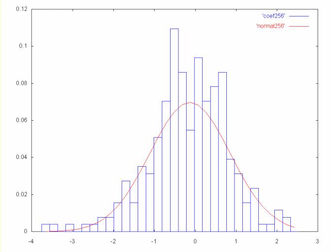
class bell_curves
Plot the Haar coefficients as a histogram, in Gnuplot format. In
another file generate a normal curve with the mean and standard
deviation of the histogram. Using two files allows the histogram
and the normal curve to be plotted together using gnu plot, where
the histogram and normal curve will be different colored lines.
If the spectrum as 256 coefficient points, the files generated
would be coef256 and normal256 for the coefficient
histogram and the normal curve. To plot these using gnuplot the
following command would be used:
This will result in a gnuplot graph where the histogram is one
color and the normal curve is another.
A normal curve is a probability distribution, where the values
are plotted on the x-axis and the probability of that value
occuring is plotted on the y-axis. To plot the coefficient
histogram in the same terms, the percentage of the total points
is represented for each histogram bin. This is the same as the
integral of the normal curve in the histogram range, if the
coefficient histogram fell in a perfect normal distribution.
For example;
Calculate the mean and standard deviation.
The stddev function is passed an array of numbers.
It returns the mean, standard deviation in the
bell_info object.
normal_interval
Numerically integreate the normal curve with mean
info.mean and standard deviation info.sigma
over the range low to high.
There normal curve equation that is integrated is:
Where u is the mean and s is the standard deviation.
The area under the section of this curve from low to
high is returned as the function result.
The normal curve equation results in a curve expressed as
a probability distribution, where probabilities are expressed
as values greater than zero and less than one. The total area
under a normal curve is one.
The integral is calculated in a dumb fashion (e.g., we're not
using anything fancy like simpson's rule). The area in
the interval xi to xi+1
is
Where the function g(xi) is the point on the
normal curve probability distribution at xi.
Output a gnuplot formatted histogram of the area under a normal
curve through the range m.low to m.high based on the
mean and standard deviation of the values in the array v.
The number of bins used in the histogram is num_bins
Write out a histogram for the Haar coefficient frequency
spectrum in gnuplot format.
plot_freq
Generate histograms for a set of coefficients
(passed in the argument v). Generate
a seperate histogram for a normal curve. Both
histograms have the same number of bins and the
same scale.
The histograms are written to separate files in gnuplot
format. Different files are needed (as far as I can tell)
to allow different colored lines for the coefficient histogram
and the normal plot. The file name reflects the number of
points in the coefficient spectrum.
This function is passed an ordered set of Haar wavelet
coefficients. For each frequency of coefficients
a graph will be generated, in gnuplot format, that
plots the ordered Haar coefficients as a histogram. A
gaussian (normal) curve with the same mean and standard
deviation will also be plotted for comparision.
The histogram for the coefficients is generated by counting the
number of coefficients that fall within a particular bin range and
then dividing by the total number of coefficients. This results in
a histogram where all bins add up to one (or to put it another way,
a curve whose area is one).
The standard formula for a normal curve results in a curve showing
the probability profile. To convert this curve to the same
scale as the coefficient histogram, the area under the curve is
integrated over the range of each bin (corresponding to the
coefficient histogram bins). The area under the normal curve
is one, resulting in the same scale.
The size of the coefficient array must be a power of two. When the
Haar coefficients are ordered (see inplace_haar) the coefficient
frequencies are the component powers of two. For example, if the
array length is 512, there will be 256 coefficients from the highest
frequence from index 256 to 511. The next frequency set will
be 128 in length, from 128 to 255, the next will be 64 in length
from 64 to 127, etc...
As the number of coefficients decreases, the histograms become
less meaningful. This function only graphs the coefficient
spectrum down to 64 coefficients.
class bell_curves
Plot the Haar coefficients as a histogram, in Gnuplot format. In
another file generate a normal curve with the mean and standard
deviation of the histogram. Using two files allows the histogram
and the normal curve to be plotted together using gnu plot, where
the histogram and normal curve will be different colored lines.
If the spectrum as 256 coefficient points, the files generated
would be coef256 and normal256 for the coefficient
histogram and the normal curve. To plot these using gnuplot the
following command would be used:
This will result in a gnuplot graph where the histogram is one
color and the normal curve is another.
A normal curve is a probability distribution, where the values
are plotted on the x-axis and the probability of that value
occuring is plotted on the y-axis. To plot the coefficient
histogram in the same terms, the percentage of the total points
is represented for each histogram bin. This is the same as the
integral of the normal curve in the histogram range, if the
coefficient histogram fell in a perfect normal distribution.
Calculate the mean and standard deviation.
The stddev function is passed an array of numbers.
It returns the mean, standard deviation in the
bell_info object.
normal_interval
Numerically integreate the normal curve with mean
info.mean and standard deviation info.sigma
over the range low to high.
There normal curve equation that is integrated is:
Where u is the mean and s is the standard deviation.
The area under the section of this curve from low to
high is returned as the function result.
The normal curve equation results in a curve expressed as
a probability distribution, where probabilities are expressed
as values greater than zero and less than one. The total area
under a normal curve is one.
The integral is calculated in a dumb fashion (e.g., we're not
using anything fancy like simpson's rule). The area in
the interval xi to xi+1
is
Where the function g(xi) is the point on the
normal curve probability distribution at xi.
Output a gnuplot formatted histogram of the area under a normal
curve through the range m.low to m.high based on the
mean and standard deviation of the values in the array v.
The number of bins used in the histogram is num_bins
Write out a histogram for the Haar coefficient frequency
spectrum in gnuplot format.
plot_freq
Generate histograms for a set of coefficients
(passed in the argument v). Generate
a seperate histogram for a normal curve. Both
histograms have the same number of bins and the
same scale.
The histograms are written to separate files in gnuplot
format. Different files are needed (as far as I can tell)
to allow different colored lines for the coefficient histogram
and the normal plot. The file name reflects the number of
points in the coefficient spectrum.
This function is passed an ordered set of Haar wavelet
coefficients. For each frequency of coefficients
a graph will be generated, in gnuplot format, that
plots the ordered Haar coefficients as a histogram. A
gaussian (normal) curve with the same mean and standard
deviation will also be plotted for comparision.
The histogram for the coefficients is generated by counting the
number of coefficients that fall within a particular bin range and
then dividing by the total number of coefficients. This results in
a histogram where all bins add up to one (or to put it another way,
a curve whose area is one).
The standard formula for a normal curve results in a curve showing
the probability profile. To convert this curve to the same
scale as the coefficient histogram, the area under the curve is
integrated over the range of each bin (corresponding to the
coefficient histogram bins). The area under the normal curve
is one, resulting in the same scale.
The size of the coefficient array must be a power of two. When the
Haar coefficients are ordered (see inplace_haar) the coefficient
frequencies are the component powers of two. For example, if the
array length is 512, there will be 256 coefficients from the highest
frequence from index 256 to 511. The next frequency set will
be 128 in length, from 128 to 255, the next will be 64 in length
from 64 to 127, etc...
As the number of coefficients decreases, the histograms become
less meaningful. This function only graphs the coefficient
spectrum down to 64 coefficients.
Calculate floor( log2( val ) ), where val > 0
The log function is undefined for 0.
@param val
a positive value
@return floor( log2( val ) )
*/
public static byte log2(int val )
{
byte log;
for (log = 0; val > 0; log++, val = val >> 1)
;
log--;
return log;
} // log2
/**
nearestPower2
Given a value "val", where val > 0, nearestPower2 returns
the power of 2 that is less than or equal to val.
*/
public static int nearestPower2( int val )
{
byte l = log2( val );
int power = power2( l );
return power;
} // nearestPower2
} // class binary
�����������������������������������������������������������������������������������������������������������������������������������������������������������������������������������������������������������������������������������������������������������������������������������������������������������������������������������������������������������������������������������wavelets/wavelet_util/coef_spectrum.java������������������������������������������������������������100644 � 1040 � 1001 � 10327 7321421413 17330� 0����������������������������������������������������������������������������������������������������ustar ���������������������������������everyone���������������������������������������������������������������������������������������������������������������������������������������������������������������������������������������������������������������
package wavelet_util;
import wavelets.*;
import java.io.*;
/**
After the wavelet transform is calculated, regenerate the time
series with a given spectrum set to zero, or with all but a given
spectrum set to zero. The plots are generated from the highest
frequency spectrum to the lower frequency spectrums. The
highest frequency spectrum is left out of later plots since
this spectrum contains most of the noise.
Wavelets allow a time series to be examined by
filtering the component spectrum. For example, the
Haar wavelet transform can be calculated and the
highest frequency spectrum of coefficients can
be set to zero. When the reverse Haar transform
is calculated, the time series will be regenerated
without this spectrum.
Wavelets can also be used to look at a single
spectrum in isolation. This can be done by
setting all but the one spectrum to zero and
then regenerating the time series. This will
result in a time series showning the contribution
of that spectrum.
Moving from the high frequency coefficient spectrum
to the lower frequency spectrum, set each spectrum
to zero and output the regenerated time series to
a file.
The highest frequency spectrum contains most of the
noise so when subsequent spectrum are set to zero,
the highest frequency spectrum is not included.
Moving from high frequency to lower frequency, regenerate
the time series from only one spectrum.
Note that coef[0] contains the time series average and
must exist for all coefficient arrays in order to
regenerate the time series.
Define the class gnuplot3D for the wavelet_util package.
The class outputs a Haar wavelet spectrum array in a format
that can be read by gnuplot for 3D plotting. This function
can be used to plot either Haar wavelet spectrums or
Haar wavelet coefficients.
The constructor is given an array of Haar spectrum values and
a file name. The Haar spectrum values will be written out
to the file so that they can be graphed.
The length of the array must be 2N. The lengths
of the spectrums are 2N-1, ... 20.
If the original data was
The Haar spectrum will be:
If the original data length was 2N, then the total
length of the spectrum data will be 2N-1, so the
first element is zeroed out in the case of a Haar spectrum.
In the case of the wavelet coefficients, the first value will
be the average for the entire sample. In either case this
value will not be output.
The plot used to display the Haar wavelet spectrums is modeled after
the plots shown in Robi Polikar's Wavelet
Tutorial, Part III. Here the x-axis represents the offset in the
data. The y-axis represents the width of the Haar window (which will
be a power of two) and the z-axis represents the spectrum value.
In order for gnuplot to display a 3D surface each line must have the
same number of points. The wavelet spectrum is graphed over the
original rage. The first spectrum repeats two values for each
average or coefficient calculated. The second spectrum repeats
each value four times, the third spectrum eight times, etc...
The objective in filtering is to remove noise while keeping the
features that are interesting.
Wavelets allow a time series to be examined at various
resolutions. This can be a powerful tool in filtering out noise.
This class supports the subtraction of gaussian noise from
the time series.
The identification of noise is complex and I have not found any
material that I could understand which discussed noise
identification in the context of wavelets. I did find some material
that has been difficult and frustrating. In particular
Image Processing and Data Analysis: the multiscale approach
by Starck, Murtagh and Bijaoui.
If the price of a stock follows a random walk, its price will be
distributed in a bell (gaussian) curve. This is one way of stating
the concept from financial theory that the daily return is normally
distributed (here daily return is defined as the difference between
yesterdays close price and today's close price). Movement outside
the bounds of the curve may represent something other than a random walk
and so, in theory, might be interesting.
At least in the case of the single test case used in developing this
code (Applied Materials, symbol: AMAT), the coefficient distribution
in the highest frequency is almost a perfect normal curve. That is,
the mean is close to zero and the standard deviation is close to
one. The area under this curve is very close to one. This
resolution approximates the daily return. At lower frequencies the
mean moves away from zero and the standard deviation increases.
This results is a flattened curve, whose area in the coefficient
range is increasingly less than one.
The code in this class subtracts the normal curve from the
coefficients at each frequency up to some minimum. This leaves only
the coefficients above the curve which are used to regenerate the
time series (without the noise, in theory). This filter removes 50
to 60 percent of the coefficients.
Its probably worth mentioning that there are other kinds of
noise, most notably Poisson noise. In theory daily data
tends to show gaussian noise, while intraday data would
should Poisson noise. Intraday Poisson noise would result
from the random arrival and size of orders.
This function has two public methods:
n
filter_time_series, which is passed a file name and a time series
gaussian_filter which is passed a set of Haar coefficient
spectrum and an array allocated for the noise values. The
noise array will be the same size as the coefficient array.
a1
c1
c2 c3
c4 c5 c6 c7
a1 = a1 + c1
a2 = a1 - c1

a1 = a1 + c2
a2 = a1 - c2
a3 = a2 + c3
a4 = a2 - c3

a1 = a1 + c4
a2 = a1 - c4
a3 = a2 + c5
a4 = a2 - c5
a5 = a3 + c6
a6 = a3 - c6
a7 = a4 + c7
a8 = a4 - c7
5.0
-3.0
0.0 -1.0
1.0 -2.0 1.0 0.0

5.0+(-3), 5.0-(-3) = {2 8}

2+0, 2-0, 8+(-1), 8-(-1) = {2, 2, 7, 9}

2+1, 2-1, 2+(-2), 2-(-2), 7+1, 7-1, 9+0, 9-0 = {3,1,0,4,8,6,9,9}
     t1 = a1 + c1;
     t2 = a1 - c1;
     a1 = t1;
     c1 = t2
start: {5.0, -3.0, 0.0, -1.0, 1.0, -2.0, 1.0, 0.0}
[0, 1]
L = 1
{2.00, 8.01, 0.0, -1.0, 1.0, -2.0, 1.0, 0.0}
 sort:

 start: {2.00, 8.01, 0.0, -1.0, 1.0, -2.0, 1.0, 0.0}
[0, 2], [1, 3]
L = 2
{2.00, 7.02, 2.01, 9.03, 1.0, -2.0, 1.0, 0.0}
 sort:
exchange [1, 2]
{2.00, 2.01, 7.02, 9.03, 1.0, -2.0, 1.0, 0.0}

 start: {2.0, 2.0, 7.0, 9.0, 1.0, -2.0, 1.0, 0.0}
[0, 4], [1, 5], [2, 6], [3, 7]
L = 4
{3.00, 0.02, 8.04, 9.06, 1.01, 4.03, 6.05, 9.07}
 sort:
exchange [1, 4]
{3.00, 1.01, 8.04, 9.06, 0.02, 4.03, 6.05, 9.07}
exchange [2, 5]
{3.00, 1.01, 4.03, 9.06, 0.02, 8.04, 6.05, 9.07}
exchange [3, 6]
{3.00, 1.01, 4.03, 6.05, 0.02, 8.04, 9.06, 9.07}
exchange [2, 4]
{3.00, 1.01, 0.02, 6.05, 4.03, 8.04, 9.06, 9.07}
exchange [3, 5]
{3.00, 1.01, 0.02, 8.04, 4.03, 6.05, 9.06, 9.07}
exchange [3, 4]
{3.00, 1.01, 0.02, 4.03, 8.04, 6.05, 9.06, 9.07}
********/
private void inverse_ordered() {
int len = wavefx.length;
for (int L = 1; L < len; L = L * 2) {
int i;
// calculate
for (i = 0; i < L; i++) {
int a_ix = i;
int c_ix = i + L;
double a1 = wavefx[a_ix] + wavefx[c_ix];
double a1_plus_1 = wavefx[a_ix] - wavefx[c_ix];
wavefx[a_ix] = a1;
wavefx[c_ix] =a1_plus_1;
} // for i
// sort
int offset = L-1;
for (i = 1; i < L; i++) {
for (int j = i; j < L; j++) {
double tmp = wavefx[j];
wavefx[j] = wavefx[j+offset];
wavefx[j+offset] = tmp;
} // for j
offset = offset - 1;
} // for i
} // for L
} // inverse_ordered
/**
*
        new_ai = ai + ci
        new_ai+1 = ai - ci
a0 c0 c1 c0 c2 c0 c1 c0

a1 = a0 + c2
a1 = a0 - c2

a1 c0 c1 c0 a1 c0 c1 c0

a2 = a1 + c1
a2 = a1 - c1
a2 = a1 + c1
a2 = a1 - c1

a2 c0 a2 c0 a2 c0 a2 c0

a3 = a2 + c0
a3 = a2 - c0
a3 = a2 + c0
a3 = a2 - c0
a3 = a2 + c0
a3 = a2 - c0
a3 = a2 + c0
a3 = a2 - c0

a3 a3 a3 a3 a3 a3 a3 a3
50  10  01 -20 -32  10 -11  00

a1 = 5 + (-3) = 2
a1 = 5 - (-3) = 8

21  10  01 -20 81  10 -11  00

a2 = 2 + 0    = 2
a2 = 2 - 0    = 2
a2 = 8 + (-1) = 7
a2 = 8 - (-1) = 9

22  10  22 -20 72  10 92  00

a3 = 2 + 1    = 3
a3 = 2 - 1    = 1
a3 = 2 + (-2) = 0
a3 = 2 - (-2) = 4
a3 = 7 + 1    = 8
a3 = 7 - 1    = 6
a3 = 9 + 0    = 9
a3 = 9 - 0    = 9

33  13  03  43  83  63  93  93
      HaarStep = (S0 + S1)/2  // average of S0 and S1
      HaarWave = (S0 - S1)/2  // average difference of S0 and S1
Copyright and Use
This software was written and is copyrighted by Ian Kaplan, Bear
Products International, www.bearcave.com, 2001.
iank@bearcave.com
*/
public class simple_haar extends wavelet_base {
private double haar_value; // the final Haar step value
private Vector coef; // The Haar coefficients
private double[] data;
/**
*
data[0] = 5.0;
wavelet:
{[5.0];
-3.0;
0.0, -1.0;
1.0, -2.0, 1.0, 0.0}

tmp = d[0];
d[0] = tmp + c[0, 0]
d[4] = tmp - c[0, 0]

tmp = d[0];
d[0] = tmp + c[1, 0]
d[2] = tmp - c[1, 0]
tmp = d[4];
d[4] = tmp + c[1, 1]
d[6] = tmp - c[1, 1]

tmp = d[0];
d[0] = tmp + c[2, 0]
d[1] = tmp - c[2, 0]
tmp = d[2];
d[2] = tmp + c[2, 1]
d[3] = tmp - c[2, 1]
tmp = d[4];
d[4] = tmp + c[2, 2]
d[5] = tmp - c[2, 2]
tmp = d[6];
d[6] = tmp + c[2, 3]
d[7] = tmp - c[2, 3]
*/
public void inverse() {
if (data != null && coef != null && coef.size() > 0) {
int len = data.length;
data[0] = haar_value;
if (len > 0) {
// System.out.println("inverse()");
byte log = binary.log2( len );
len = binary.power2( log ); // calculation must be on 2 ** n values
int vec_ix = 0;
int last_p = 0;
byte p_adj = 1;
for (byte l = (byte)(log-1); l >= 0; l--) {
int p = binary.power2( l );
double c[] = (double[])coef.elementAt( vec_ix );
int coef_ix = 0;
for (int j = 0; j < len; j++) {
int a_1 = p * (2 * j);
int a_2 = p * ((2 * j) + 1);
if (a_2 < len) {
double tmp = data[a_1];
data[ a_1 ] = tmp + c[coef_ix];
data[ a_2 ] = tmp - c[coef_ix];
coef_ix++;
}
else {
break;
}
} // for j
last_p = p;
p_adj++;
vec_ix++;
} // for l
}
}
} // inverse
/**
Print the simple Haar object (e.g, the
final Haar step value and the coefficients.
*/
public void pr() {
if (coef != null) {
System.out.print("{[" + haar_value + "]");
int size = coef.size();
double[] a;
for (int i = 0; i < size; i++) {
System.out.println(";");
a = (double[])coef.elementAt(i);
for (int j = 0; j < a.length; j++) {
System.out.print( a[j] );
if (j < a.length-1) {
System.out.print(", ");
}
} // for j
} // for i
System.out.println("}");
}
} // pr
/**
*
plot 'coef256' with boxes, 'normal256' with lines
f(y) = (1/(s * sqrt(2 * pi)) e-(1/(2 * s2)(y-u)2
area = (xi+1 - xi) * g(xi)
plot 'coef256' with boxes, 'normal256' with lines
f(y) = (1/(s * sqrt(2 * pi)) e-(1/(2 * s2)(y-u)2
area = (xi+1 - xi) * g(xi)
{32.0, 10.0, 20.0, 38.0, 37.0, 28.0, 38.0, 34.0,
 18.0, 24.0, 18.0,  9.0, 23.0, 24.0, 28.0, 34.0}
0.0
25.9375
29.625 22.25
25.0 34.25 17.25 27.25
21.0 29.0 32.5 36.0 21.0 13.5 23.5 31.0
The point class represents a coefficient value so that it can be sorted for histogramming and then resorted back into the orignal ordering (e.g., sorted by value and then sorted by index)
*/ private class point { point(int i, double v) { index = i; val = v; } public int index; // index in original array public double val; // coefficient value } // point /**A histogram bin
For a histogram bin bi, the range of values is bi.start to bi+1.start.
The vector object vals stores references to the point objects which fall in the bin range.
The number of values in the bin is vals.size()
*/ private class bin { bin( double s ) { start = s; } public double start; public Vector vals = new Vector(); } // bin /** Bell curve info: mean, sigma (the standard deviation) */ private class bell_info { public bell_info() {} public bell_info(double m, double s) { mean = m; sigma = s; } public double mean; public double sigma; } // bell_info /**Build a histogram from the sorted data in the pointz array. The histogram is constructed by appending a point object to the the bin vals Vector if the value of the point is between b[i].start and b[i].start + step.
*/ private void histogram( bin binz[], point pointz[] ) { double step = binz[1].start - binz[0].start; double start = binz[0].start; double end = binz[1].start; int len = pointz.length; double max = binz[ binz.length-1 ].start + step; int i = 0; int ix = 0; while (i < len && ix < binz.length) { if (pointz[i].val >= start && pointz[i].val < end) { binz[ix].vals.addElement( pointz[i] ); i++; } else { ix++; start = end; end = end + step; } } // while } // histogram /** Sort an array of point objects by the index field. */ private class sort_by_index extends generic_sort { /** if (a.index == b.index) return 0 if (a.index < b.index) return -1 if (a.index > b.index) return 1; */ protected int compare( Object a, Object b ) { int rslt = 0; point t_a = (point)a; point t_b = (point)b; if (t_a.index < t_b.index) rslt = -1; else if (t_a.index > t_b.index) rslt = 1; return rslt; } // compare } // sort_by_index /** Sort an array of point objects by the val filed. */ private class sort_by_val extends generic_sort { /** if (a.val == b.val) return 0 if (a.val < b.val) return -1 if (a.val > b.val) return 1; */ protected int compare( Object a, Object b ) { int rslt = 0; point t_a = (point)a; point t_b = (point)b; if (t_a.val < t_b.val) rslt = -1; else if (t_a.val > t_b.val) rslt = 1; return rslt; } // compare } // sort_by_val /** Allocate an array of histogram bins that is num_bins in length. Initialize the start value of each bin with a start value calculated from low and high. */ private bin[] alloc_bins( int num_bins, double low, double high ) { double range = high - low; double step = range / (double)num_bins; double start = low; bin binz[] = new bin[ num_bins ]; for (int i = 0; i < num_bins; i++) { binz[i] = new bin( start ); start = start + step; } return binz; } // alloc_bins /**Calculate the histogram of the coefficients using num_bins histogram bins
The Haar coefficients are stored in point objects which consist of the coefficient value and the index in the point array.
To calculate the histogram, the pointz array is sorted by value. After it is histogrammed it is resorted by index to return the original ordering.
*/ private bin[] calc_histo( point pointz[], int num_bins ) { // sort by value sort_by_val by_val = new sort_by_val(); by_val.sort( pointz ); int len = pointz.length; double low = pointz[0].val; double high = pointz[len-1].val; bin binz[] = alloc_bins( num_bins, low, high ); histogram( binz, pointz ); // return the array to its original order by sorting by index sort_by_index by_index = new sort_by_index(); by_index.sort( pointz ); return binz; } // calc_histo /**Allocate and initialize an array of point objects. The size of the array is end - start. Each point object in the array is initialized with its index and a Haar coefficient (from the coef array).
Since the allocation code has to iterate through the coefficient spectrum the mean and standard deviation are also calculated to avoid an extra iteration. These values are returned in the bell_info object.
*/ private point[] alloc_points( double coef[], int start, int end, bell_info info ) { int size = end - start; point pointz[] = new point[ size ]; double sum = 0; int ix = start; for (int i = 0; i < size; i++) { pointz[i] = new point( i, coef[ix] ); sum = sum + coef[ix]; ix++; } double mean = sum / (double)size; // now calculate the standard deviation double stdDevSum = 0; double x; for (int i = 0; i < size; i++) { x = pointz[i].val - mean; stdDevSum = stdDevSum + (x * x); } double sigmaSquared = stdDevSum / (size-1); double sigma = Math.sqrt( sigmaSquared ); info.mean = mean; info.sigma = sigma; return pointz; } // alloc_points /**normal_interval
Numerically integreate the normal curve with mean info.mean and standard deviation info.sigma over the range low to high.
There normal curve equation that is integrated is:
f(y) = (1/(s * sqrt(2 * pi)) e-(1/(2 * s2)(y-u)2
Where u is the mean and s is the standard deviation.
The area under the section of this curve from low to high is returned as the function result.
The normal curve equation results in a curve expressed as a probability distribution, where probabilities are expressed as values greater than zero and less than one. The total area under a normal curve with a mean of zero and a standard deviation of one is is one.
The integral is calculated in a dumb fashion (e.g., we're not using anything fancy like simpson's rule). The area in the interval xi to xi+1 is
area = (xi+1 - xi) * g(xi)
where the function g(xi) is the point on the normal curve probability distribution at xi.
@param info This object encapsulates the mean and standard deviation @param low Start of the integral @param high End of the integral @param num_points Number of points to calculate (should be even) */ private double normal_interval(bell_info info, double low, double high, int num_points ) { double integral = 0; if (info != null) { double s = info.sigma; // calculate 1/(s * sqrt(2 * pi)), where s is the stddev double sigmaSqrt = 1.0 / (s * (Math.sqrt(2 * Math.PI))); double oneOverTwoSigmaSqrd = 1.0 / (2 * s * s); double range = high - low; double step = range / num_points; double x = low; double f_of_x; double area; double t; for (int i = 0; i < num_points-1; i++) { t = x - info.mean; f_of_x = sigmaSqrt * Math.exp( -(oneOverTwoSigmaSqrd * t * t) ); area = step * f_of_x; // area of one rectangle in the interval integral = integral + area; // sum of the rectangles x = x + step; } // for } return integral; } // normal_interval /**Set num_points values in the histogram bin b to zero. Or, if the number of values is less than num_zero, set all values in the bin to zero.
The num_zero argument is derived from the area under the normal curve in the histogram bin interval. This area is a fraction of the total curve area. When multiplied by the total number of coefficient points we get num_zero.
The noise coefficients are preserved (returned) in the noise array argument.
*/ private void zero_points( bin b, int num_zero, double noise[] ) { int num = b.vals.size(); int end = num_zero; if (end > num) end = num; point p; for (int i = 0; i < end; i++) { p = (point)b.vals.elementAt( i ); noise[ p.index ] = p.val; p.val = 0; } } // zero_points /**Subtract the gaussian (or normal) curve from the histogram of the coefficients. This is done by integrating the gaussian curve over the range of a bin. If the number of items in the bin is less than or equal to the area under the curve in that interval, all items in the bin are set to zero. If the number of items in the bin is greater than the area under the curve, then a number of bin items equal to the curve area is set to zero.
The area under a normal curve is always less than or equal to one. So the area returned by normal_interval is the fraction of the total area. This is multiplied by the total number of coefficients.
The function returns the number of coefficients that are set to zero (e.g., the number of coefficients that fell within the gaussian curve). These coefficients are the noise coefficients. The noise coefficients are returned in the noise argument.
*/ private int subtract_gauss_curve( bin binz[], bell_info info, int total_points, double noise[] ) { int points_in_interval = total_points / binz.length; double start = binz[0].start; double end = binz[1].start; double step = end - start; double percent; int num_points; int total_zeroed = 0; for (int i = 0; i < binz.length; i++) { percent = normal_interval( info, start, end, points_in_interval ); num_points = (int)(percent * (double)total_points); total_zeroed = total_zeroed + num_points; if (num_points > 0) { zero_points( binz[i], num_points, noise ); } start = end; end = end + step; } // for return total_zeroed; } // subtract_gauss_curve /**This function is passed the section of the Haar coefficients that correspond to a single spectrum. It compares this spectrum to a gaussian curve and zeros out the coefficients within the gaussian curve.
The function returns the number of points filtered out as the function result. The noise spectrum is also returned in the noise argument.
*/ private int filter_spectrum( double coef[], int start, int end, double noise[] ) { final int num_bins = 32; int num_filtered; bell_info info = new bell_info(); point pointz[] = alloc_points( coef, start, end, info ); bin binz[] = calc_histo( pointz, num_bins ); num_filtered = subtract_gauss_curve( binz, info, pointz.length, noise ); int zero_count = 0; // copy filtered coefficients back into the coefficient array int ix = start; for (int i = 0; i < pointz.length; i++) { coef[ix] = pointz[i].val; ix++; } return num_filtered; } // filter_spectrum /** Normalize the noise array to zero by subtracting the smallest value from all points. */ private void normalize_to_zero( double noise[] ) { double min = noise[0]; for (int i = 1; i < noise.length; i++) { if (min > noise[i]) min = noise[i]; } // for // normalize for (int i = 0; i < noise.length; i++) { noise[i] = noise[i] - min; } } // normalize_to_zero /**This function is passed a set of Haar wavelet coefficients that result from the Haar wavelet transform. It applies a gaussian noise filter to each frequency spectrum. This filter zeros out coefficients that fall within a gaussian curve. This alters the input data (the coef array).
The coef argument is the input argument and contains the coefficients. The noise argument is an output argument and contains the coefficients that have been filtered out. This allows a noise spectrum to be rebuilt.
*/ public void gaussian_filter( double coef[], double noise[] ) { final int min_size = 64; // minimum spectrum size int total_filtered = 0; int num_filtered; int end = coef.length; int start = end >> 1; while (start >= min_size) { num_filtered = filter_spectrum( coef, start, end, noise ); total_filtered = total_filtered + num_filtered; end = start; start = end >> 1; } // Note that coef[0] is the average across the // time series. This value is needed to regenerate // the noise spectrum time series. noise[0] = coef[0]; System.out.println("gaussian_filter: total points filtered out = " + total_filtered ); } // gaussian_filter /** Calculate the Haar tranform on the time series (whose length must be a factor of two) and filter it. Then calculate the inverse transform and write the result to a file whose name is file_name. A noise spectrum is written to file_name_noise. */ public void filter_time_series( String file_name, double ts[] ) { double noise[] = new double[ ts.length ]; wavelets.inplace_haar haar = new wavelets.inplace_haar(); haar.wavelet_calc( ts ); haar.order(); gaussian_filter( ts, noise ); haar.inverse(); PrintWriter prStr = OpenFile( file_name ); if (prStr != null) { for (int i = 0; i < ts.length; i++) { prStr.println( i + " " + ts[i] ); } prStr.close(); } if (noise != null) { // calculate the inverse Haar function for the noise haar.setWavefx( noise ); haar.setIsOrdered(); haar.inverse(); normalize_to_zero( noise ); // write the noise spectrum out to a file prStr = OpenFile( file_name + "_noise" ); if (prStr != null) { for (int i = 0; i < noise.length; i++) { prStr.println( i + " " + noise[i] ); } prStr.close(); } } } // filter_time_series } // noise_filter ��������������������������������������������������������������������wavelets/wavelet_util/plot.java���������������������������������������������������������������������100644 � 1040 � 1001 � 763 7317254147 15430� 0����������������������������������������������������������������������������������������������������ustar ���������������������������������everyone��������������������������������������������������������������������������������������������������������������������������������������������������������������������������������������������������������������� package wavelet_util; import java.io.*; public abstract class plot { abstract String class_name(); public PrintWriter OpenFile( String path ) { PrintWriter prStr = null; try { FileOutputStream outStr = new FileOutputStream( path ); prStr = new PrintWriter( outStr ); } catch (Exception e) { System.out.println( class_name() + ": file name = " + path + ", " + e.getMessage() ); } return prStr; } // OpenFile } // plot �����������������������������������������������������������������������������������������������������������������������������������������������������������������������������������������������������������������������������������������������������������������������������������������������������������������������������������������������������������������������������������������������������������������������������������������������������������������������������������������������������������������������������������������������������������������������������������������������������������������������������������������������������������������������������������������������������������������������������������������������������������������������������������������������������������������������������������������������������������������������������������������������������������������������������������������������������������������������������������������������������������������������������������������������������������������������������