A stationary signal is a signal that repeats into infinity with the same periodicity.
One of the assumptions of the Fourier transform is that the sample of the signal over which the Fourier transform is calculated is large to be representative. To be representative the sample should capture at least one period of all the components that make up the signal. The Fourier transform assumes that the signal is stationary and that the signals in the sample continue into infinity. The Fourier transform performs poorly when this is not the case.
For example, the Java code below generates a sample where the signal doubles in frequency every 2pi.
    float pi = (float)Math.PI;
    float sampleRate = 512;
    float range = (float)4.0f * (2.0f * pi);
    float step = range/sampleRate;

    Vector data = new Vector();

    float scale = 1;
    float cnt = 0.0f;
    for (double x = 0; x <= range; x = x + step) {
      float y = (float)(Math.sin( scale * x));
      point p = new point((float)x, y);
      cnt = cnt + step;
      if (cnt > (2 * pi)) {
	cnt = 0.0f;
	scale = scale + scale;
      }
      data.addElement( p );
    }
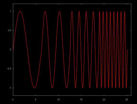
As the graph below shows, this results in a signal that is stationary within blocks of 2pi. However, the signal abruptly doubles in frequency on the 2pi boundary.
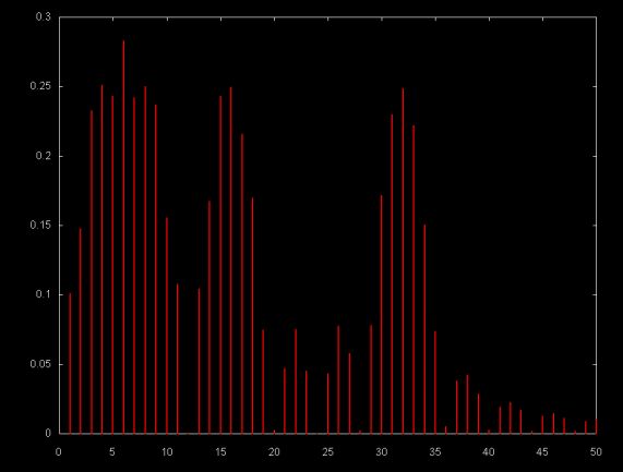
Since this signal is not stationary, at least within the sample window, the DFT magnitude plot below does a poor job of resolving the frequencies.
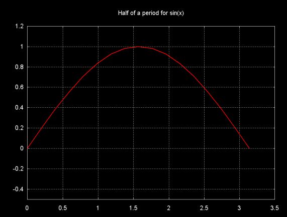
A similar problem can exist if the sample window on which the DFT is calculated is not large enough. The graph below shows a sample that consists of a half a period of a sin(x) signal.
The graph below shows the DFT magnitude plot for a sample consisting of a half period of sin(x).
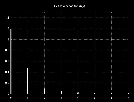
Note that the major magnitude line is at frequency zero. This sample does contains only a half of a sin(x) period. Although sin(x) is an infinite, stationary, signal, the DFT "sees" only the partial period, so a zero frequency results. The other frequency lines are a result of DFT leakage.
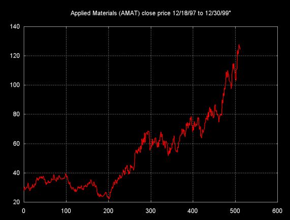
Fourier transforms can be applied to any time series, including non-stationary, non-smooth time series. For example, the graph below shows a 512 day close price time series for the stock Applied Materials (symbol AMAT).
There continues to be an argument about whether stationary signals can be found in financial time series. A number of software packages for financial analysists and traders include Fourier transforms, in addition to statistical and linear modeling functions. Compared to the Fourier transform, wavelet techniques are relatively new, but wavelet transforms are being incorporated into a few packages as well.
There is a huge body of literature on "technical trading" which attempts to recognize stationarity in financial time series. The fact that some of these techniques make money lends support to technical trading in general. It is unlikely that all technical trading techniques are equally valid.
Even in the case of signals that lend themselves well to Fourier analysis, the issue of stationarity depends on the size of the sample window. As the half period sin(x) plot demonstrates, whether the DFT recognizes a signal as stationary depends in part on the window size. There are those who argue that in the right time frame, financial signals show stationarity. So can the Fourier transform be used to uncover stationary components in a financial time series? The Fourier transform of the AMAT close price time series is shown below.
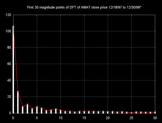
Note that the major magnitude component is at frequency zero and represents the magnitude of the graph. Small signal components (and probably DFT leakage) are spread throughout the DFT results. In theory there might be smaller magnitude stationary waves embedded in this time series, but it is difficult to tell whether the magnitudes at at 3, 5, 9 are DFT leakage artifacts or actual signal components.
As Lyons notes, log plots show more detail for the small magnitude components of the signal. This is shown in the graph below, where the y-axis uses a log scale. The graph uses both magnitude lines (red) and a line through the points (magenta). While this graphs shows more detail, it is still not clear whether these small magnitudes are actually signal components or artifacts. The fact that they are so small suggests that they are artifacts.
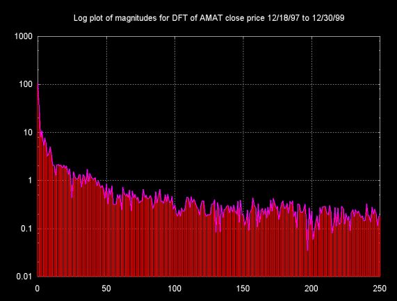
The ambiguous results and the extent of the DFT leakage artifacts are one of the reasons that wavelets perform better for non-stationary and non-smooth time series.
Ian Kaplan, September 2001
Revised:
Back to A Notebook Compiled While Reading Understanding Digital Signal Processing by Lyons
